-
Kernix Lab,
Publié le 21/06/2016
Deep learning attempts to model data through multiple processing layers containing non-linearities. It has proved very efficient in classifying images, as shown by the impressive results of deep neural networks on the ImageNet Competition for example. However, training these models requires very large datasets and is quite time consuming.
So in this tutorial, we will show how it is possible to obtain very good image classification performance with a pre-trained deep neural network that will be used to extract relevant features and a linear SVM that will be trained on these features to classify the images. We will use TensorFlow, Google’s deep learning system that was open sourced last November, and scikit-learn.

This tutorial shows an example of transfer learning: a deep neural network that is highly efficient on some task should be useful for solving related problems. Here we will use a network developed by Google, the Inception-v3, that has been trained on some images (the ImageNet dataset) to extract relevant features on another dataset that does not include the same categories.
We will classify images from the Product Image Categorization Dataset.
This dataset contains images of products from different categories collected on MSN shopping, such as baby shoes or skates for example. Images are 100 x 100 pixels and they are labelled with their category.
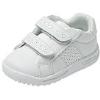
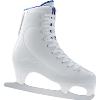
This dataset is interesting because it contains some categories of products that are not present in the ImageNet dataset, such as hiking backpacks for example.
For this tutorial, we selected 48 categories (out of the 100 available), in order to reduce computation time. These categories were selected based on their similarity (e.g. different kind of shoes) in order to increase the complexity of the classification task.
In this section we will extract features from images using a pre-trained deep learning model.
We will use the following Python librairies :
import os
import re

import tensorflow as tf
import tensorflow.python.platform
from tensorflow.python.platform import gfile
import numpy as np
import pandas as pd
import sklearn
from sklearn import cross_validation
from sklearn.metrics import accuracy_score, confusion_matrix
from sklearn.svm import SVC, LinearSVC
import matplotlib.pyplot as plt
%matplotlib inline
import pickle
The pre-trained deep learning model that will be used is Inception-v3. It has been developed by Google and has been trained for the ImageNet Competition using the data from 2012. We chose this model because of its high classification performance and because it is easily available in TensorFlow.
To download this model into the tutorial directory, you should run in a terminal:
cd tensorflow/models/image/imagenet python classify_image.py --model_dir TUTORIAL_DIR/imagenet
The pre-trained model will be in the imagenet directory within your tutorial directory. The images are assumed to be in the images directory within your tutorial directory.
model_dir = 'imagenet'
images_dir = 'images/'
list_images = [images_dir+f for f in os.listdir(images_dir) if re.search('jpg|JPG', f)]
To use TensorFlow, you should define a graph that represents the description of computations. Then these computations will be executed within what is called sessions. If you want to know more about the basics of TensorFlow, you can go here.
The following function creates a graph from the graph definition that we just downloaded and that is saved in classify_image_graph_def.pb
def create_graph():
with gfile.FastGFile(os.path.join(
model_dir, 'classify_image_graph_def.pb'), 'rb') as f:
graph_def = tf.GraphDef()
graph_def.ParseFromString(f.read())
_ = tf.import_graph_def(graph_def, name='')
Then, the next step is to extract relevant features.
To do so, we retrieve the next-to-last layer of the Inception-v3 as a feature vector for each image. Indeed, the last layer of the convolutional neural network corresponds to the classification step: as it has been trained for the ImageNet dataset, the categories that it will be output will not correspond to the categories in the Product Image Classification dataset we are interested in.
The output of the next-to-last layer, however, corresponds to features that are used for the classification in Inception-v3. The hypothesis here is that these features can be useful for training another classification model, so we extract the output of this layer. In TensorFlow, this layer is called pool_3.
The following function returns the features corresponding to the output of this next-to-last layer and the labels for each image.
def extract_features(list_images):
nb_features = 2048
features = np.empty((len(list_images),nb_features))
labels = []

create_graph()

with tf.Session() as sess:

next_to_last_tensor = sess.graph.get_tensor_by_name('pool_3:0')

for ind, image in enumerate(list_images):
if (ind%100 == 0):
print('Processing %s...' % (image))
if not gfile.Exists(image):
tf.logging.fatal('File does not exist %s', image)

image_data = gfile.FastGFile(image, 'rb').read()
predictions = sess.run(next_to_last_tensor,
{'DecodeJpeg/contents:0': image_data})
features[ind,:] = np.squeeze(predictions)
labels.append(re.split('_\d+',image.split('/')[1])[0])

return features, labels
features,labels = extract_features(list_images)
Then the features and labels are saved, so they can be used without re-running this step that can be quite long (about 30 min on my laptop with 4 cores and 16 Go RAM).
pickle.dump(features, open('features', 'wb'))
pickle.dump(labels, open('labels', 'wb'))
We will now use the features that we just computed with TensorFlow to train a classifier on the images. Another strategy could be to re-train the last layer of the CNN in TensorFlow, as shown here in TensorFlow tutorials and here for the python version.
features = pickle.load(open('features'))
labels = pickle.load(open('labels'))
We will use 80% of the data as the training set and 20% as the test set.
X_train, X_test, y_train, y_test = cross_validation.train_test_split(features, labels, test_size=0.2, random_state=42)
Following scikit-learn’s machine learning map, we chose to use a linear SVM to classify the images into the 48 categories using the features computed with TensorFlow. We used the LinearSVC implementation with the default parameters.
clf = LinearSVC(C=1.0, loss='squared_hinge', penalty='l2',multi_class='ovr')
clf.fit(X_train, y_train)
y_pred = clf.predict(X_test)
We will plot the confusion matrix (computed with scikit-learn) to visualize the classification performance, on top of the accuracy score.
def plot_confusion_matrix(y_true,y_pred):
cm_array = confusion_matrix(y_true,y_pred)
true_labels = np.unique(y_true)
pred_labels = np.unique(y_pred)
plt.imshow(cm_array[:-1,:-1], interpolation='nearest', cmap=plt.cm.Blues)
plt.title("Confusion matrix", fontsize=16)
cbar = plt.colorbar(fraction=0.046, pad=0.04)
cbar.set_label('Number of images', rotation=270, labelpad=30, fontsize=12)
xtick_marks = np.arange(len(true_labels))
ytick_marks = np.arange(len(pred_labels))
plt.xticks(xtick_marks, true_labels, rotation=90)
plt.yticks(ytick_marks,pred_labels)
plt.tight_layout()
plt.ylabel('True label', fontsize=14)
plt.xlabel('Predicted label', fontsize=14)
fig_size = plt.rcParams["figure.figsize"]
fig_size[0] = 12
fig_size[1] = 12
plt.rcParams["figure.figsize"] = fig_size
print("Accuracy: {0:0.1f}%".format(accuracy_score(y_test,y_pred)*100))
plot_confusion_matrix(y_test,y_pred)
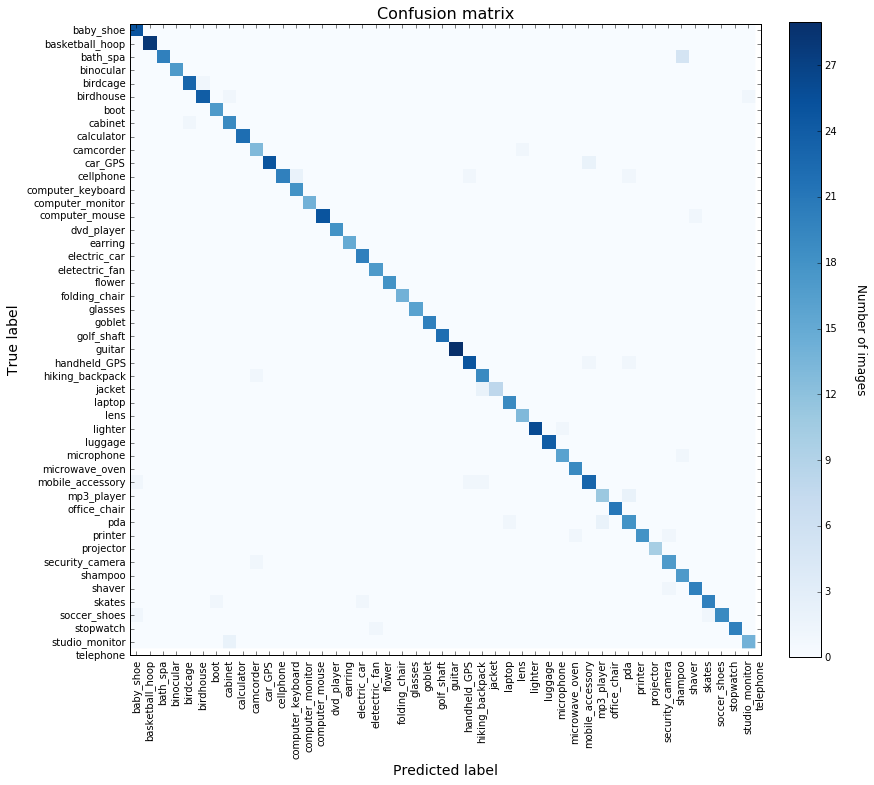
The classification accuracy is 95.4 % on the test set, which is quite impressive, especially as it does not require so much work on our side !
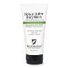
It is interesting to look at the confusion matrix to try to understand the errors. We can see that bath_spa images are sometimes misclassified as shampoo. This is not so surprising when you see examples of these categories :

This approach is interesting as we obtain very good classification accuracy with only a few lines of code and in about 30 minutes on a laptop.
Although we could have obtained even better results with a fully trained deep neural network, this result highlights that the features extracted by Inception-v3 on the new images are highly relevant, even if the images used for the training were pretty different.
Note however that the images used in this example were very clean, well centered, of the same size…When analyzing datasets in real life, it is often a lot messier, so it might require quite a lot of preprocessing to obtain satisfying results and the classification accuracy is likely to be lower.

In one of our projects with ERDF, we successfully developed an approach similar to the one presented in this tutorial to classify pictures of electrical equipments.
