-
Kernix Lab,
-
Data scientist
Publié le 01/04/2016
From purchase suggestions on e-commerce websites to content customization on multimedia platforms, recommender systems happen to be more and more widespread among the web.
Modern companies such as Facebook, Netflix, Amazon all develop their own, aiming to propose items or contents which are more personalized and relevant to their users.
The designation « recommender system » embrace a wide set of solutions, each of which has its own advantages and limitations. Usually, one has to combine several different strategies to address a given issue. Nowadays, there are almost as many ways of classifying the different methods as data scientists around the world. A great synthesis of the different families of methods is however available on this blog. The most famous one is probably the so-called « collaborative filtering« , in which the user is asked to give information about his personal tastes, usually in the form of ratings. The system then aims to predict what rating the user would give to a new item. The idea of « predicting » naturally brings model-based solutions exploiting machine learning.
There exists many alternatives to machine learning recommender systems. Obviously there are ways of predicting ratings which don’t necessarily require the use of sophisticated machine learning models. For example, predicting the rating one user would give to one item as the mean rating attributed to this item by a subset of similar users often brings surprisingly accurate results. Besides, there sometimes is no need to predict ratings in order to retrieve efficient suggestions. Depending on the purpose of the recommender system, simply proposing the most popular items may do the job.
In this tutorial, we propose a straightforward implementation of a recommender system taking advantage of a graph database. In such a database, information is stored as nodes, which are linked together by edges. This allows to easily retrieve knowledge about relationships between nodes. Therefore, graph databases are useful to describe systems of strongly connected entities, such as social networks or metro networks for example. At Kernix, we benefit from experts in graph-related topics who manipulate such databases everyday. Please find here our latest publication about Neo4j, which is an open-source graph database implemented in Java. It is accessible from softwares written in other languages using the Cypher Query Language. Neo4j can be downloaded from here.

In what follows, we will restrain ourselves to a concrete example : recommending movies to one user, using a database of movie ratings and knowing the ratings the user we’re interested in gave to a subset of movies. You’ll be successively guided through all the steps allowing to build the graph database, add a new user and perform personalized recommendations.
Three complementary strategies will be implemented. To evaluate their respective performances, we asked a film-lover (named « guinea pig » in the following) to choose some movies among the dataset and attribute its own ratings. We then computed recommendations with each of the three strategies and asked our guinea pig to give ratings to the suggested movies he had actually already seen. In the end, the performances of our recommender systems will also be qualitatively compared to a model-based collaborative filtering method which has proven to be quite effective for addressing that kind of issues. Here is the outline of this tutorial:
We will use the ML-100k dataset gathered by GroupLens Research on the MovieLens website. This dataset consists in 100,000 ratings (1-5) from 943 users on 1682 movies. The dataset has been cleaned up such
that each user has rated at least 20 movies. Data is gathered in the form of a set of DSV files, the description of which is available here.
As regards the MovieLens dataset, it can be represented in the form of a very simple graph, with :
First, one has to build the graph database from the DSV files describing the dataset. For Python users, the py2neo package enables to read and write into the Neo4j database. Once Neo4j is installed, the command « sudo neo4j start » will launch Neo4j on port 7474. The graph can then be visualized in a browser at the address : http://localhost:7474/.
To access the graph database from an ipython notebook, import the Graph module from py2neo and create a new instance of Graph. The argument passed in the Graph() function is the path to the graph database :
import pandas as pd
import numpy as np
import matplotlib as plt
from py2neo import Graph

%matplotlib inline
graph = Graph('http://neo4j:neo4j@localhost:7474/db/data/')
Load the DSV files which contain useful data :
# Loading user-related data
user = pd.read_csv('ml-100k/u.user', sep='|', header=None, names=['id','age','gender','occupation','zip code'])
n_u = user.shape[0]

# Loading genres of movies
genre = pd.read_csv('ml-100k/u.genre', sep='|', header=None, names=['name', 'id'])
n_g = genre.shape[0]

# Loading item-related data
# Format : id | title | release date | | IMDb url | "genres"
# where "genres" is a vector of size n_g : genres[i]=1 if the movie belongs to genre i
movie_col = ['id', 'title','release date', 'useless', 'IMDb url']
movie_col = movie_col + genre['id'].tolist()
movie = pd.read_csv('ml-100k/u.item', sep='|', header=None, names=movie_col)
movie = movie.fillna('unknown')
n_m = movie.shape[0]

# Loading ratings
rating_col = ['user_id', 'item_id','rating', 'timestamp']
rating = pd.read_csv('ml-100k/u.data', sep='\t' ,header=None, names=rating_col)
n_r = rating.shape[0]
Once the files are loaded, we can build step by step the graph database :
##### Create the nodes relative to Users, each one being identified by its user_id #####
# "MERGE" request : creates a new node if it does not exist already
tx = graph.cypher.begin()
statement = "MERGE (a:`User`{user_id:{A}}) RETURN a"
for u in user['id']:
    tx.append(statement, {"A": u})

tx.commit()


##### Create the nodes relative to Genres, each one being identified by its genre_id, and with the property name #####
tx = graph.cypher.begin()
statement = "MERGE (a:`Genre`{genre_id:{A}, name:{B}}) RETURN a"
for g,row in genre.iterrows() :
    tx.append(statement, {"A": row.iloc[1], "B": row.iloc[0]})

tx.commit()
##### Create the Movie nodes with properties movie_id, title and url  then create the Is_genre edges #####
tx = graph.cypher.begin()
statement1 = "MERGE (a:`Movie`{movie_id:{A}, title:{B}, url:{C}}) RETURN a"
statement2 = ("MATCH (t:`Genre`{genre_id:{D}}) "
              "MATCH (a:`Movie`{movie_id:{A}, title:{B}, url:{C}}) MERGE (a)-[r:`Is_genre`]->(t) RETURN r")

# Looping over movies m
for m,row in movie.iterrows() :
    # Create "Movie" node
    tx.append(statement1, {"A": row.loc['id'], "B": row.loc['title'].decode('latin-1'), "C": row.loc['IMDb url']})
    # is_genre : vector of size n_g, is_genre[i]=True if Movie m belongs to Genre i
    is_genre = row.iloc[-19:]==1
    related_genres = genre[is_genre].axes[0].values

    # Looping over Genres g which satisfy the condition : is_genre[i]=True
    for g in related_genres :
        # Retrieve node corresponding to genre g, and create relation between g and m
        tx.append(statement2,\
                  {"A": row.loc['id'], "B": row.loc['title'].decode('latin-1'), "C": row.loc['IMDb url'], "D": g})

    # Every 100 movies, push queued statements to the server for execution to avoid one massive "commit"
    if m%100==0 : tx.process()

# End with a "commit"
tx.commit()


##### Create the Has_rated edges, with rating as property #####
tx = graph.cypher.begin()
statement = ("MATCH (u:`User`{user_id:{A}}) "
             "MATCH (m:`Movie`{movie_id:{C}}) MERGE (u)-[r:`Has_rated`{rating:{B}}]->(m) RETURN r")

# Looping over ratings
for r,row in rating.iterrows() :
    # Retrieve "User" and "Movie" nodes, and create relationship with the corresponding rating as property
    tx.append(statement, {"A": row.loc['user_id'], "B": row.loc['rating'], "C": row.loc['item_id']})
    if r%100==0 : tx.process()

tx.commit()
At this point, it is important to create an index on each type of nodes. This will dramatically reduce the time needed to query the database.
graph.cypher.execute('CREATE INDEX ON :User(user_id)')
graph.cypher.execute('CREATE INDEX ON :Movie(movie_id)')
graph.cypher.execute('CREATE INDEX ON :Genre(genre_id)')
To add a new user in the graph database, create your own DSV file containing the ratings he gave to a subset of movies, in the form : movie_id | rating. Below is a shown a part of the file describing our guinea pig’s tastes :
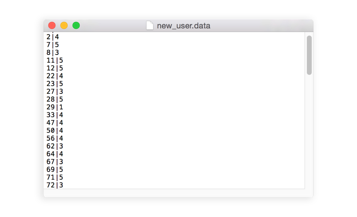
Then merge the data related to the new user into the graph database :
n_u = n_u + 1
new_user_id = n_u

# Create the node corresponding to the new user
tx = graph.cypher.begin()
statement = "MERGE (a:`User`{user_id:{A}}) RETURN a"
tx.append(statement, {"A": new_user_id})
tx.commit()

# Load ratings from new user
new_ratings = pd.read_csv('ml-100k/new_user.data', sep='|', header=None, names=['item_id', 'rating'])
n_r = n_r + new_ratings.shape[0]

# Create Has_rated relations between new user and movies
tx = graph.cypher.begin()
statement = ("MATCH (u:`User`{user_id:{A}}) "
           "MATCH (m:`Movie`{movie_id:{C}}) MERGE (u)-[r:`Has_rated`{rating:{B}}]->(m) RETURN r")
for r,row in new_ratings.iterrows() :
  tx.append(statement, {"A": new_user_id, "B": row.loc['rating'], "C": row.loc['item_id']})
  if r%100==0 : tx.process()

tx.commit()
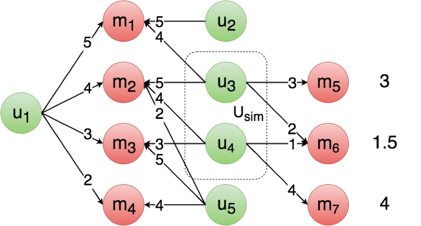
In what follows, we will implement three complementary collaborative-filtering strategies in the so-called « user-based » paradigm. This means we’ll focus on the past behaviour of users (« what did they watch? », « what ratings did they attribute? ») to highlight subsets of users who are similar to one another. To perform a recommendation for one given user u1, the global behaviour of all its similar users will be studied. Here are the different steps :
For each of the three strategies, we asked our guinea pig to attribute ratings afterwards to the top 20 suggestions in order to qualitatively evaluate their performances.
The first strategy consists in considering the similarity between two users u1 and u2 as the ratio of the number of movies they have in common, over the number of movies
u1 has seen. As regards movies seen by similar users, they are ranked from most popular to least popular. This simple method can be implemented even if ratings are not known.


The threshold t can be optimized to tune the selectivity of a subset of similar users, and at the same time the average number of users in Usim.


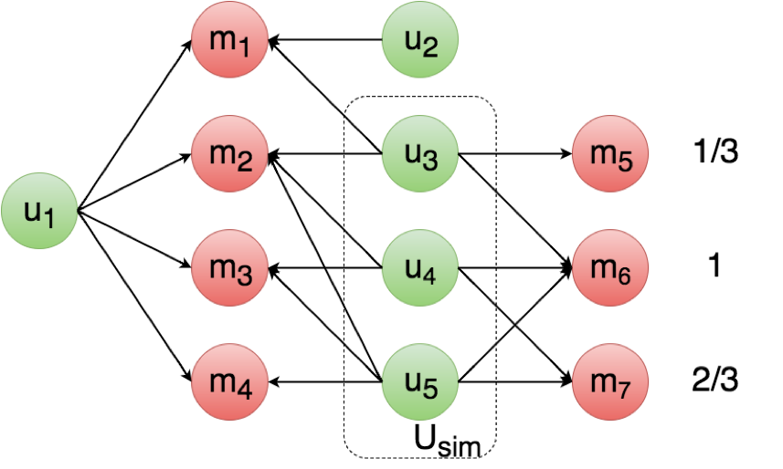
A schematic representation of strategy 1
The py2neo/Cypher query allowing to retrieve the recommendations for our guinea pig (user_id = 944) is:
user_id = 944
threshold = 0.5

# In Strategy 1, the similarity between two users u1 and u2 is the proportion of movies they have in common
# The score of one given movie m is the proportion of users similar to u1 who rated m

query = (### Similarity normalization : count number of movies seen by u1 ###
  # Count movies rated by u1 as countm
  'MATCH (u1:`User` {user_id:{user_id}})-[:`Has_rated`]->(m1:`Movie`) '
  'WITH count(m1) as countm '
  ### Score normalization : count number of users who are considered similar to u1 ###
  # Retrieve all users u2 who share at least one movie with u1
  'MATCH (u1:`User` {user_id:{user_id}})-[:`Has_rated`]->(m1:`Movie`) '
  'MATCH (m1)<-[r:`Has_rated`]-(u2:`User`) '
  'WHERE NOT u2=u1 '
  # Compute similarity
  'WITH u2, countm, tofloat(count(r))/countm as sim '
  # Keep users u2 whose similarity with u1 is above some threshold
  'WHERE sim>{threshold} '
  # Count number of similar users as countu
  'WITH count(u2) as countu, countm '
  ### Recommendation ###
  # Retrieve all users u2 who share at least one movie with u1
  'MATCH (u1:`User` {user_id:{user_id}})-[:`Has_rated`]->(m1:`Movie`) '
  'MATCH (m1)<-[r:`Has_rated`]-(u2:`User`) '
  'WHERE NOT u2=u1 '
  # Compute similarity
  'WITH u1, u2,countu, tofloat(count(r))/countm as sim '
  # Keep users u2 whose similarity with u1 is above some threshold
  'WHERE sim>{threshold} '
  # Retrieve movies m that were rated by at least one similar user, but not by u1
  'MATCH (m:`Movie`)<-[r:`Has_rated`]-(u2) '
  'WHERE NOT (m)<-[:`Has_rated`]-(u1) '
  # Compute score and return the list of suggestions ordered by score
  'RETURN DISTINCT m, tofloat(count(r))/countu as score ORDER BY score DESC ')
tx = graph.cypher.begin()
tx.append(query, {'user_id': user_id, 'threshold': threshold})
result = tx.commit()
The graph structure allows to retrieve the set of users similar to u1, without browsing the whole set of users. Likewise, the set of movies seen by the similar users but not by u1 can be retrieved in a very simple and direct way, which makes graph databases well suited for that kind of approaches.
The top 20 recommended movies for our guinea pig and their approximate scores are listed below. Figures in the third column correspond to the ratings the guinea pig gave afterwards :
| Title | Score | Rating |
|---|---|---|
| The Fugitive (1993) | 0.93 | – |
| Indiana Jones and the Last Crusade (1989) | 0.90 | 5 |
| E.T. the Extra-Terrestrial (1982) | 0.90 | 4 |
| The Princess Bride (1987) | 0.85 | – |
| The Blues Brother (1980) | 0.82 | – |
| When Harry Met Sally… (1989) | 0.82 | – |
| Mission: Impossible (1996) | 0.82 | 5 |
| Dead Poets Society (1989) | 0.82 | – |
| Star Trek: The Wrath of Khan (1982) | 0.81 | not interested |
| Jaws (1975) | 0.80 | 5 |
| The Hunt for Red October (1990) | 0.80 | 4 |
| True Lies (1994) | 0.79 | 4 |
| Star Trek: First Contact (1996) | 0.79 | not interested |
| Speed (1994) | 0.78 | 3 |
| Die Hard (1988) | 0.78 | 5 |
| Batman (1989) | 0.77 | 5 |
| Raising Arizona (1987) | 0.76 | – |
| 2001: A Space Odyssey (1968) | 0.76 | 4 |
| Star Trek IV: The Voyage Home (1986) | 0.75 | not interested |
| A Fish Called Wanda (1988) | 0.75 | 4 |
One can notice that the worst rating the guinea pig gave is 3, which means that even if the recommendations aren’t a « perfect match » to his tastes, this simple and easy-to-implement strategy still allows to retrieve quite relevant recommendations. However, not taking into account ratings given by users leads to not really personalized recommendations based only on popularity-related considerations. Consequently, three different Star Trek movies are suggested to our guinea pig while he is actually not interested at all in the Star Trek universe, contrary to his set of similar users who often watch these movies.
In strategy 2, we propose to refine the way movies are ranked by exploiting the ratings given by the subset of similar users.

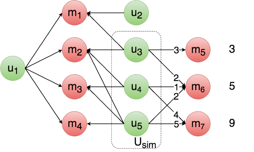
A schematic representation of strategy 2
The py2neo/Cypher query allowing to retrieve the recommendations for our guinea pig (user_id = 944) is :
user_id = 944
threshold = 0.5

# In Strategy 2, the similarity between two users u1 and u2 is the proportion of movies they have in common
# The score of one movie m is the sum of ratings given by users similar to u1

query = (### Similarity normalization : count number of movies seen by u1 ###
    # Count movies rated by u1 as countm
    'MATCH (m1:`Movie`)<-[:`Has_rated`]-(u1:`User` {user_id:{user_id}}) '
    'WITH count(m1) as countm '
    ### Recommendation ###
    # Retrieve all users u2 who share at least one movie with u1
    'MATCH (u2:`User`)-[r2:`Has_rated`]->(m1:`Movie`)<-[r1:`Has_rated`]-(u1:`User` {user_id:{user_id}}) '
    'WHERE (NOT u2=u1) AND (abs(r2.rating - r1.rating) <= 1) '
    # Compute similarity
    'WITH u1, u2, tofloat(count(DISTINCT m1))/countm as sim '
    # Keep users u2 whose similarity with u1 is above some threshold
    'WHERE sim>{threshold} '
    # Retrieve movies m that were rated by at least one similar user, but not by u1
    'MATCH (m:`Movie`)<-[r:`Has_rated`]-(u2) '
    'WHERE (NOT (m)<-[:`Has_rated`]-(u1)) '
    # Compute score and return the list of suggestions ordered by score
    'RETURN DISTINCT m,tofloat(sum(r.rating)) as score ORDER BY score DESC ')

tx = graph.cypher.begin()
tx.append(query, {'user_id': user_id, 'threshold': threshold})
result = tx.commit()
The top 20 recommended movies and their scores are listed below. Figures on the right correspond to the ratings the guinea pig gave afterwards :
| Title | Score | Rating |
|---|---|---|
| The Fugitive (1993) | 289 | – |
| The Princess Bride (1987) | 284 | – |
| E.T. the Extra-Terrestrial (1982) | 265 | 4 |
| Indiana Jones and the Last Crusade (1989) | 264 | 5 |
| Jaws (1975) | 262 | 5 |
| Dead Poets Society (1989) | 259 | – |
| The Blues Brother (1980) | 257 | – |
| Die Hard (1988) | 257 | 5 |
| Raising Arizona (1987) | 253 | – |
| When Harry Met Sally… (1989) | 250 | – |
| The Hunt for Red October (1990) | 248 | 4 |
| Stand By Me (1986) | 247 | – |
| Schindler’s List (1993) | 243 | 5 |
| 2001: A Space Odyssey (1968) | 241 | 4 |
| Star Trek: The Wrath of Khan (1982) | 240 | not interested |
| One Flew Over the Cuckoo’s Nest (1975) | 237 | 5 |
| A Fish Called Wanda (1988) | 237 | 4 |
| Get Shorty (1995) | 232 | – |
| Speed (1994) | 229 | 3 |
| True Lies (1994) | 229 | 4 |
Here, exploiting the ratings given by similar users to rank movies introduces a notion of « quality » on top of popularity-related considerations. The Star Trek-related suggestions are then ranked less highly : only one remains in the top 20 recommendations. Strategies 1 and 2 are very rough as regards the evaluation of similarity : two users are considered similar provided that they have a sufficient amount of movies in common, but their respective tastes are actually not compared. In strategy 3, we propose a more accurate way of finding similar users, and a ranking method which allows to recommend movies that are not necessarily popular.
In strategy 3, users are considered similar if they have a sufficient amount of movies in common AND if they have often given approximatively the same ratings to these movies.


user_id = 944
threshold = 0.5

# In Strategy 3, the similarity between two users is the proportion of movies for which they gave almost the same rating
# The score of one movie m is the mean rating given by users similar to u1

query = (### Similarity normalization : count number of movies seen by u1 ###
    # Count movies rated by u1 as countm
    'MATCH (m1:`Movie`)<-[:`Has_rated`]-(u1:`User` {user_id:{user_id}}) '
    'WITH count(m1) as countm '
    ### Recommendation ###
    # Retrieve all users u2 who share at least one movie with u1
    'MATCH (u2:`User`)-[r2:`Has_rated`]->(m1:`Movie`)<-[r1:`Has_rated`]-(u1:`User` {user_id:{user_id}}) '
    # Check if the ratings given by u1 and u2 differ by less than 1
    'WHERE (NOT u2=u1) AND (abs(r2.rating - r1.rating) <= 1) '
    # Compute similarity
    'WITH u1, u2, tofloat(count(DISTINCT m1))/countm as sim '
    # Keep users u2 whose similarity with u1 is above some threshold
    'WHERE sim>{threshold} '
    # Retrieve movies m that were rated by at least one similar user, but not by u1
    'MATCH (m:`Movie`)<-[r:`Has_rated`]-(u2) '
    'WHERE (NOT (m)<-[:`Has_rated`]-(u1)) '
    # Compute score and return the list of suggestions ordered by score
    'WITH DISTINCT m, count(r) as n_u, tofloat(sum(r.rating)) as sum_r '
    'WHERE n_u > 1 '
    'RETURN m, sum_r/n_u as score ORDER BY score DESC')

tx = graph.cypher.begin()
tx.append(query, {'user_id': user_id, 'threshold': threshold})
result = tx.commit()
| Title | Score | Rating |
|---|---|---|
| Hard Eight (1996) | 5.0 | – |
| Traveller (1997) | 5.0 | – |
| Some Folks Call It a Sling Blade (1993) | 4.87 | – |
| The Sweet Hereafter (1997) | 4.80 | – |
| Paths of Glory (1957) | 4.71 | 5 |
| Wallace & Gromit (1996) | 4.69 | 4 |
| Love in the Afternoon (1957) | 4.66 | – |
| The Wrong Trousers (1993) | 4.65 | – |
| Kundun (1997) | 4.60 | – |
| Schindler’s List (1993) | 4.58 | 5 |
| Waiting for Guffman (1996) | 4.57 | – |
| Casablanca (1942) | 4.52 | 5 |
| The Double Life of Veronique (1991) | 4.50 | – |
| Shall We Dance? (1996) | 4.50 | 4 |
| The Horseman on the Roof (1995) | 4.50 | 5 |
| Rear Window (1954) | 4.50 | 5 |
| Double Happiness (1994) | 4.50 | – |
| Eve’s Bayou (1997) | 4.50 | – |
| Secrets & Lies (1996) | 4.47 | – |
| One Flew Over the Cuckoo’s Nest (1975) | 4.47 | 5 |
| R5 | R4 | R3 | |
|---|---|---|---|
| Strategy 1 | 45% | 45% | 9% |
| Strategy 2 | 45% | 45% | 9% |
| Strategy 3 | 75% | 25% | 0% |
The substantial increase in R5 from strategies 1 and 2 to strategy 3, as well as R3 dropping to 0, reveals that strategy 3 grabs better the new user’s personal tastes. This comes from the fact that in strategy 3, we impose that two users must have close enough tastes to be considered similar. As a result, the subset of users considered similar to our guinea pig is more restrictive compared to strategies 1 and 2.
![]()
where X is a (nm x n)-matrix, each line of which describes one given movie m in terms of n parameters. Θ is a (nu x n)-matrix each line of which grabs the personal tastes of user ni. As the elements of X and Θ are learned simultaneously, each modification of the database -either adding a new user or adding a new movie- requires to train the whole model once again. For this reason, such an approach is much more time-consuming.
The top 20 suggestions out of a matrix-factorization model are listed below :
| Title | Rating |
|---|---|
| Chinatown (1974) | 5 |
| Sunset Blvd. (1950)) | – |
| The Princess Bride (1987) | – |
| Dr Strangelove (1963) | 5 |
| The Manchurian Candidate (1962) | – |
| Secrets & Lies (1996) | – |
| North by Northwest (1959) | 4 |
| To Kill a Mockingbird (1962) | – |
| Das Boot (1981) | 5 |
| Lawrence of Arabia (1962) | 5 |
| 12 Angry Men (1957) | – |
| Some Folks Call It a Sling Blade (1993) | – |
| Wallace & Gromit (1996) | 4 |
| Schindler’s List (1993) | 5 |
| The Third Man (1949) | – |
| Rear Window (1954) | 5 |
| One Flew Over the Cuckoo’s Nest (1975) | 5 |
| The Wrong Trousers (1993) | – |
| A Close Shave (1995) | – |
| Casablanca (1942) | 5 |
The values of Rn obtained for the model-based recommender system are listed below :
| R5 | R4 | R3 | |
|---|---|---|---|
| Model-based | 80% | 20% | 0% |
Those values confirm that this kind of approach grabs well one user’s personal tastes. The values of Rn obtained for strategy 3 and for this model-based recommender system are quite close to each other. This shows that strategy 3 allows to reach a degree of customization comparable to a model-based approach while requiring much less computation time.
In light of the values of Rn, one might think that strategy 3 is the « best » of the three strategies we introduced. However, defining what would be the ideal set of suggestions constitutes a hot topic, and is actually quite tricky. The key-question is : what does the user actually expect from our recommender system? The answer might not necessarily be « Recommend only movies that I would have rated 5/5 ». What about movies he would have given a lower rating, but that are very popular among his friends? Wouldn’t he be interested in these movies?
What’s more, the increase in accuracy in reproducing someone’s personal tastes happens to be done at the cost of serendipity: the more the suggestions stick to someone’s taste, the less the algorithm is prone to recommend unexpected contents that the user would never have found by himself.
As the three strategies discussed above offer different degrees of customization, combining them allows to get a balance between suggesting contents that look alike what the user usually watches, and still being able to make a « happy accident ».
In this tutorial, we implemented three complementary strategies in the user-based paradigm : the tastes of one given user are infered from the behaviour of its similar users (« What did similar users watch? », « What ratings did they attribute? »). The subsets of similar users are identified based on their past behaviour (« They watched the same movies », « They approximately gave the same ratings »).
In the next tutorial, we’ll propose to enhance our recommender system by exploiting an item-based method, which consists in highlighting subsets of similar items (movies in our case) instead of similar users. In particular, we’ll introduce semantic analysis as a way to evaluate the similarity between two movies. It will then be possible to recommend movies that are most similar to the movies one given user has already watched.
