-
Kernix Lab,
-
Data scientist
Publié le 09/02/2017
In our previous article – Image classification with a pre-trained deep neural network -, we introduced a quick guide on how to build an image classifier, using a pre-trained neural network to perform feature extraction and plugging it into a custom classifier that is specifically trained to perform image recognition on the dataset of interest.
The present article is meant to unveil the details that are hidden inside the « black box » represented by a neural network built for image classification. We propose to build a basic convolutional neural network so as to grab the key concepts behind it, and at the same time become familiar with the Python Keras library for neural networks.
In our previous article, the feature extraction was performed with the deep Inception-V3 trained on the ImageNet dataset which contains millions of images, yielding a classification accuracy of 95.4% on the Product Image Categorization Dataset. Unfortunately, this dataset is no longer public, that’s why here we propose to use the CIFAR-10 dataset which is composed of 60000 32×32 RGB images, distributed among 10 classes, with 6000 images per class. Three years ago, a Kaggle competition was held, aiming to yield the best classification accuracy on this dataset. The competition winner, Ben Graham, reached an accuracy of 95.5% by using a deep convolutional network the architecture of which is described here.
The architecture of the model introduced in this tutorial will be kept very basic on purpose, to allow the training and parameter tuning to be carried out on a regular computer using CPU. For this reason, obviously our toy model won’t allow us to get such an impressive performance, but let’s see what accuracy we can reach!
Over the past few years, neural nets have proven to be very efficient as regards image classification. As an example, « basic » multilayer perceptrons can yield very good results in terms of classification errors on the well-known handwritten digits MNIST dataset (ref : D. C. Ciresan et al. (2010))
To get familiar with neural networks (with a nice tutorial on the handwritten digits classification problem) : http://neuralnetworksanddeeplearning.com/chap1.html
Object recognition using « real life » images can however prove to be tricky, and this for many reasons. A few are listed below :
Because of their particular properties, convolutional neural networks (CNNs) allow to address the issues listed above.
By construction, CNNs are well suited for image classification :
Some useful references to gain knowledge of CNNs : http://cs231n.github.io/convolutional-networks/
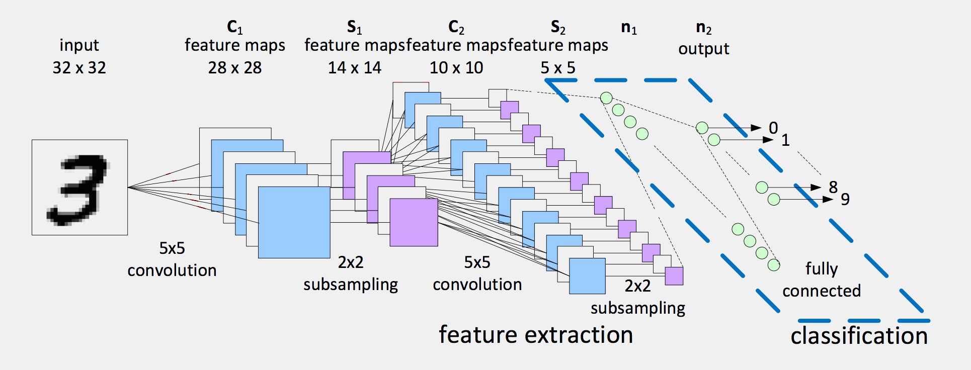
A basic CNN consists in successions of convolutional layers (CL) and pooling layers (PL). Convolutional layers allow to extract several feature maps from the input images, while pooling layers perform some subsampling (i.e. dimensionality reduction) on the feature maps. Those successions of CLs and PLs correspond to a step of feature extraction. For image classification, the output layer is a fully connected NN layer with a number of units equal to the number of classes. The output layer activation function is a softmax, so that the ith output unit activation is consistent with the probability that the image belongs to class i.
It’s also common to see in a CNN, the CLs and PLs being combined with some rectification (non-linearities) and normalization layers that can drastically improve the classification accuracy (Jarrett et al. (2009))
The following scheme, taken from M. Peemen et al. (2011), represents a basic architecture with two convolution+subsampling steps plugged into a classifier :
Below are loaded some useful libraries for building, training and evaluating neural nets.
from __future__ import print_function

import os
import re

import numpy as np
import PIL
from PIL import Image

from scipy.stats import randint as sp_randint

import matplotlib.pyplot as plt

from sklearn.base import BaseEstimator
from sklearn.preprocessing import LabelEncoder
from sklearn.cross_validation import StratifiedShuffleSplit
from sklearn.cross_validation import cross_val_score
from sklearn.model_selection import train_test_split
from sklearn.model_selection import GridSearchCV, RandomizedSearchCV
from sklearn.metrics import classification_report, confusion_matrix

from keras.models import Sequential
from keras.layers import Dense, Convolution2D, AveragePooling2D, MaxPooling2D, Flatten, Activation
from keras.callbacks import EarlyStopping
from keras.utils import np_utils
from keras.datasets import cifar10

%matplotlib inline
The piece of code below allows to load the CIFAR-10 dataset directly from the Keras library. To do so, the cifar10 module has to be imported from keras.datasets.
In the following, the model architecture selection and hyperparameter tuning will be performed by 3-fold cross-validation on the train set (X_train, y_train). The test set is staged for performance assessment of the model chosen in the end.
(X_train, y_train), (X_test, y_test) = cifar10.load_data()
print('Train set size : ', X_train.shape[0])
print('Test set size : ', X_test.shape[0])
Below the X_train and X_test arrays are reshaped to match 2D matrices. This is because some of the scikit-learn methods that will be used later (for example RandomizedSearchCV) assume this particular shape for the input features. The X_train and X_test 2D matrices will however be reshaped to take their original format (n_examples, height, width, n_channels) before being fed into the convolutional network.
y_train = y_train.flatten()
y_test = y_test.flatten()
n_labels = len(np.unique(y_train))

n_train = X_train.shape[0]
n_test = X_test.shape[0]
height= X_train.shape[1]
width = X_train.shape[2]
n_channels = X_train.shape[3]
print(n_train, n_test, height, width, n_channels)

X_train = X_train.reshape((n_train,height*width*n_channels))
X_test = X_test.reshape((n_test,height*width*n_channels))

print(X_train.shape, y_train.shape)
print(X_test.shape, y_test.shape)
The pipeline to perform model selection is inspired from the reference article Jarrett et al. (2009).
In this paper, the impact of the following model attributes on object classification accuracy is investigated :
Jarrett et al. (2009) state that, in general, the best suited architecture consists in using at least two successive convolution+pooling+rectification steps for feature extraction. In general, max pooling provides slightly better results than average pooling. As regards the rectification layers, many functions can be used but in what follows we’ll stick to rectified linear units (ReLU), as those are the ones that are often the best suited for image classification.
Still, we encourage you to play by yourself with those different parameters to test if the best model architecture that you find is consistent with what Jarrett et al. (2009) claims !
We’ll first use the most basic classifier which consists in a single fully connected output layer with 10 units (because we have 10 classes) and a softmax activation function. This corresponds to a linear classifier. Then we’ll add an hidden layer between the feature extractor and the output layer, leading to more complex decision boundaries.
Some hyperparameters tuning will be performed by using randomized search. The concerned hyperparameters are :
def unit_test(classifier, nb_iter=3):
test_size = 0.2
random_state = 15
cv = StratifiedShuffleSplit(y_train, nb_iter,test_size=test_size,random_state=random_state)
clf = classifier()
scores = cross_val_score(clf, X=X_train, y=y_train, scoring='accuracy', cv=cv)
return scores
def hyperparameter_optim(classifier, params, nb_iter=10, cv=3):

clf = RandomizedSearchCV(estimator=classifier(), param_distributions=params, n_iter=nb_iter, cv=cv, scoring='accuracy')
clf.fit(X_train, y_train)

print("Best parameters set found:")
print(clf.best_params_)
print()
print("Grid scores:")
means = clf.cv_results_['mean_test_score']
stds = clf.cv_results_['std_test_score']
for mean, std, params in zip(means, stds, clf.cv_results_['params']):
print("%0.3f (+/-%0.03f) for %r"
       % (mean, std * 2, params))
print()

return clf
class Classifier(BaseEstimator):

def __init__(self, nb_filters=32, filter_size=3, pool_size=2):
self.nb_filters = nb_filters
self.filter_size = filter_size
self.pool_size = pool_size

def preprocess(self, X):
X = X.reshape((X.shape[0],height,width,n_channels))
X = (X / 255.)
X = X.astype(np.float32)
return X

def preprocess_y(self, y):
return np_utils.to_categorical(y)

def fit(self, X, y):
X = self.preprocess(X)
y = self.preprocess_y(y)

hyper_parameters = dict(
nb_filters = self.nb_filters,
filter_size = self.filter_size,
pool_size = self.pool_size
)

print("FIT PARAMS : ")
print(hyper_parameters)

self.model = build_model(hyper_parameters)

earlyStopping = EarlyStopping(monitor='val_loss', patience=1, verbose=1, mode='auto')
self.model.fit(X, y, nb_epoch=20, verbose=1, callbacks=[earlyStopping], validation_split=0.2,
              validation_data=None, shuffle=True)
return self

def predict(self, X):
X = self.preprocess(X)
return self.model.predict_classes(X)

def predict_proba(self, X):
X = self.preprocess(X)
return self.model.predict(X)

def score(self, X, y):
print(self.model.evaluate(self, X, y, batch_size=32, verbose=1, sample_weight=None))
return self.model.evaluate(self, X, y, batch_size=32, verbose=1, sample_weight=None)
def build_model(hp):
net = Sequential()
net.add(Convolution2D(hp['nb_filters'], hp['filter_size'], hp['filter_size'], border_mode='same',
                 input_shape=(height,width,n_channels)))
net.add(MaxPooling2D(pool_size=(hp['pool_size'],hp['pool_size'])))
net.add(Flatten())
net.add(Dense(output_dim=n_labels))
net.add(Activation("softmax"))

net.compile(loss='categorical_crossentropy', optimizer='adadelta', metrics=['accuracy'])

return net

print(unit_test(Classifier,nb_iter=3))
This first very basic model yields a classification accuracy of 55-60%, while using max pooling. You can try to replace max by average pooling. You’ll notice that the latter yields poorer results (accuracy about 45-50%).
class Classifier(BaseEstimator):

def __init__(self, nb_filters_1=32, filter_size_1=3, pool_size_1=2,
nb_filters_2=32, filter_size_2=3, pool_size_2=2):
self.nb_filters_1 = nb_filters_1
self.filter_size_1 = filter_size_1
self.pool_size_1 = pool_size_1
self.nb_filters_2 = nb_filters_2
self.filter_size_2 = filter_size_2
self.pool_size_2 = pool_size_2

def preprocess(self, X):
X = X.reshape((X.shape[0],height,width,n_channels))
X = (X / 255.)
X = X.astype(np.float32)
return X

def preprocess_y(self, y):
return np_utils.to_categorical(y)

def fit(self, X, y):
X = self.preprocess(X)
y = self.preprocess_y(y)

hyper_parameters = dict(
nb_filters_1 = self.nb_filters_1,
filter_size_1 = self.filter_size_1,
pool_size_1 = self.pool_size_1,
nb_filters_2 = self.nb_filters_2,
filter_size_2 = self.filter_size_2,
pool_size_2 = self.pool_size_2
)

print("FIT PARAMS : ")
print(hyper_parameters)

self.model = build_model(hyper_parameters)

earlyStopping = EarlyStopping(monitor='val_loss', patience=1, verbose=1, mode='auto')
self.model.fit(X, y, nb_epoch=20, verbose=1, callbacks=[earlyStopping], validation_split=0.2,
              validation_data=None, shuffle=True)
return self

def predict(self, X):
print("PREDICT")
X = self.preprocess(X)
return self.model.predict_classes(X)

def predict_proba(self, X):
X = self.preprocess(X)
return self.model.predict(X)

def score(self, X, y):
print("SCORE")
print(self.model.evaluate(self, X, y, batch_size=32, verbose=1, sample_weight=None))
return self.model.evaluate(self, X, y, batch_size=32, verbose=1, sample_weight=None)
def build_model(hp):
net = Sequential()
net.add(Convolution2D(hp['nb_filters_1'], hp['filter_size_1'], hp['filter_size_1'], border_mode='same',
                 input_shape=(height,width,n_channels)))
net.add(Activation("relu"))
net.add(MaxPooling2D(pool_size=(hp['pool_size_1'],hp['pool_size_1'])))
net.add(Convolution2D(hp['nb_filters_2'], hp['filter_size_2'], hp['filter_size_2'], border_mode='same'))
net.add(Activation("relu"))
net.add(MaxPooling2D(pool_size=(hp['pool_size_2'],hp['pool_size_2'])))
net.add(Flatten())
net.add(Dense(output_dim=n_labels))
net.add(Activation("softmax"))

net.compile(loss='categorical_crossentropy', optimizer='adadelta', metrics=['accuracy'])

return net

print(unit_test(Classifier,nb_iter=3))
With two-steps convolutions, we go up to 66% for classification accuracy. Here the last step consists in applying a linear classifier to the features maps. Let’s try to complexify the decision boundaries.
class Classifier(BaseEstimator):

def __init__(self, nb_filters_1=32, filter_size_1=3, pool_size_1=2,
        nb_filters_2=32, filter_size_2=3, pool_size_2=2, nb_hunits=400):
self.nb_filters_1 = nb_filters_1
self.filter_size_1 = filter_size_1
self.pool_size_1 = pool_size_1
self.nb_filters_2 = nb_filters_2
self.filter_size_2 = filter_size_2
self.pool_size_2 = pool_size_2
self.nb_hunits = nb_hunits

def preprocess(self, X):
X = X.reshape((X.shape[0],height,width,n_channels))
X = (X / 255.)
X = X.astype(np.float32)
return X

def preprocess_y(self, y):
return np_utils.to_categorical(y)

def fit(self, X, y):
X = self.preprocess(X)
y = self.preprocess_y(y)

hyper_parameters = dict(
nb_filters_1 = self.nb_filters_1,
filter_size_1 = self.filter_size_1,
pool_size_1 = self.pool_size_1,
nb_filters_2 = self.nb_filters_2,
filter_size_2 = self.filter_size_2,
pool_size_2 = self.pool_size_2,
nb_hunits = self.nb_hunits
)

print("FIT PARAMS : ")
print(hyper_parameters)

self.model = build_model(hyper_parameters)

earlyStopping = EarlyStopping(monitor='val_loss', patience=1, verbose=1, mode='auto')
self.model.fit(X, y, nb_epoch=20, verbose=1, callbacks=[earlyStopping], validation_split=0.2,
              validation_data=None, shuffle=True)
return self

def predict(self, X):
print("PREDICT")
X = self.preprocess(X)
return self.model.predict_classes(X)

def predict_proba(self, X):
X = self.preprocess(X)
return self.model.predict(X)

def score(self, X, y):
print("SCORE")
print(self.model.evaluate(self, X, y, batch_size=32, verbose=1, sample_weight=None))
return self.model.evaluate(self, X, y, batch_size=32, verbose=1, sample_weight=None)
def build_model(hp):
net = Sequential()
net.add(Convolution2D(hp['nb_filters_1'], hp['filter_size_1'], hp['filter_size_1'], border_mode='same',
                 input_shape=(height,width,n_channels)))
net.add(Activation("relu"))
net.add(MaxPooling2D(pool_size=(hp['pool_size_1'],hp['pool_size_1'])))
net.add(Convolution2D(hp['nb_filters_2'], hp['filter_size_2'], hp['filter_size_2'], border_mode='same'))
net.add(Activation("relu"))
net.add(MaxPooling2D(pool_size=(hp['pool_size_2'],hp['pool_size_2'])))
net.add(Flatten())
net.add(Dense(output_dim=hp['nb_hunits']))
net.add(Activation("relu"))
net.add(Dense(output_dim=n_labels))
net.add(Activation("softmax"))

net.compile(loss='categorical_crossentropy', optimizer='adadelta', metrics=['accuracy'])

return net

print(unit_test(Classifier,nb_iter=3))
The accuracy is a bit improved (from 66% to 67%) by adding the fully connected hidden layer. Here we have arbitrarily fixed the number of hidden units to 400.
In the following cell, we’ll use randomized search to tune some hyperparameters :
This is quite time consuming (about 10 hours on a laptop with CPU), that’s why we advise you not to run directly this cell, but rather copy its content into a .py script that will be launch independantly.
def build_model(hp):
net = Sequential()
net.add(Convolution2D(hp['nb_filters_1'], hp['filter_size_1'], hp['filter_size_1'], border_mode='same',
                 input_shape=(height,width,n_channels)))
net.add(Activation("relu"))
net.add(MaxPooling2D(pool_size=(hp['pool_size_1'],hp['pool_size_1'])))
net.add(Convolution2D(hp['nb_filters_2'], hp['filter_size_2'], hp['filter_size_2'], border_mode='same'))
net.add(Activation("relu"))
net.add(MaxPooling2D(pool_size=(hp['pool_size_2'],hp['pool_size_2'])))
net.add(Flatten())
net.add(Dense(output_dim=hp['nb_hunits']))
net.add(Activation("relu"))
net.add(Dense(output_dim=n_labels))
net.add(Activation("softmax"))

net.compile(loss='categorical_crossentropy', optimizer='adadelta', metrics=['accuracy'])

return net

params = {
'nb_filters_1': [16,32,64],
'filter_size_1': [3],
'pool_size_1': [2],
'nb_filters_2': [16,32,64],
'filter_size_2': [3,6,9],
'pool_size_2': [2,4],
'nb_hunits': sp_randint(50,1000)
}
clf = hyperparameter_optim(Classifier,params, nb_iter=10)

print("Detailed classification report:")
print()
y_true, y_pred = y_test, clf.predict(X_test)
print(classification_report(y_true, y_pred))
From a randomized search performed with 15 iterations, the best set of hyperparameters that were found is :
Finally, we’ll train a model with this architecture on the whole training set and evaluate the classification accuracy on the test set (that has never been used before).
class Classifier(BaseEstimator):

def __init__(self, nb_filters_1=32, filter_size_1=3, pool_size_1=2,
        nb_filters_2=32, filter_size_2=9, pool_size_2=4, nb_hunits=750):
self.nb_filters_1 = nb_filters_1
self.filter_size_1 = filter_size_1
self.pool_size_1 = pool_size_1
self.nb_filters_2 = nb_filters_2
self.filter_size_2 = filter_size_2
self.pool_size_2 = pool_size_2
self.nb_hunits = nb_hunits

def preprocess(self, X):
X = X.reshape((X.shape[0],height,width,n_channels))
X = (X / 255.)
X = X.astype(np.float32)
return X

def preprocess_y(self, y):
return np_utils.to_categorical(y)

def fit(self, X, y):
X = self.preprocess(X)
y = self.preprocess_y(y)

hyper_parameters = dict(
nb_filters_1 = self.nb_filters_1,
filter_size_1 = self.filter_size_1,
pool_size_1 = self.pool_size_1,
nb_filters_2 = self.nb_filters_2,
filter_size_2 = self.filter_size_2,
pool_size_2 = self.pool_size_2,
nb_hunits = self.nb_hunits
)

print("FIT PARAMS : ")
print(hyper_parameters)

self.model = build_model(hyper_parameters)

earlyStopping = EarlyStopping(monitor='val_loss', patience=1, verbose=1, mode='auto')
self.model.fit(X, y, nb_epoch=20, verbose=1, callbacks=[earlyStopping], validation_split=0.2,
              validation_data=None, shuffle=True)
return self

def predict(self, X):
print("PREDICT")
X = self.preprocess(X)
return self.model.predict_classes(X)

def predict_proba(self, X):
X = self.preprocess(X)
return self.model.predict(X)

def score(self, X, y):
print("SCORE")
print(self.model.evaluate(self, X, y, batch_size=32, verbose=1, sample_weight=None))
return self.model.evaluate(self, X, y, batch_size=32, verbose=1, sample_weight=None)


def build_model(hp):
net = Sequential()
net.add(Convolution2D(hp['nb_filters_1'], hp['filter_size_1'], hp['filter_size_1'], border_mode='same',
                 input_shape=(height,width,n_channels)))
net.add(Activation("relu"))
net.add(MaxPooling2D(pool_size=(hp['pool_size_1'],hp['pool_size_1'])))
net.add(Convolution2D(hp['nb_filters_2'], hp['filter_size_2'], hp['filter_size_2'], border_mode='same'))
net.add(Activation("relu"))
net.add(MaxPooling2D(pool_size=(hp['pool_size_2'],hp['pool_size_2'])))
net.add(Flatten())
net.add(Dense(output_dim=hp['nb_hunits']))
net.add(Activation("relu"))
net.add(Dense(output_dim=n_labels))
net.add(Activation("softmax"))

net.compile(loss='categorical_crossentropy', optimizer='adadelta', metrics=['accuracy'])

return net


clf = Classifier()
clf.fit(X_train,y_train)

print("Detailed classification report:")
print()
y_true, y_pred = y_test, clf.predict(X_test)
print(classification_report(y_true, y_pred))
With our final model, we reach average precision/recall of 71%. With this very basic model, we would have ranked 65th out of 231 on the Kaggle leaderboard.
Focusing on the individual F1-scores for each class, one can notice that the labels for which performances are a bit worse (i.e. F1 < 70%) are : 2,3,4 and 5. Let’s have a look at the details of the confusion matrix to get an insight of what’s happening with those labels.
def plot_confusion_matrix(y_true,y_pred):
cm_array = confusion_matrix(y_true,y_pred)
true_labels = np.unique(y_true)
pred_labels = np.unique(y_pred)
plt.imshow(cm_array, interpolation='nearest', cmap=plt.cm.jet)
plt.title("Confusion matrix", fontsize=16)
cbar = plt.colorbar(fraction=0.046, pad=0.04)
cbar.set_label('Number of images', rotation=270, labelpad=30, fontsize=12)
xtick_marks = np.arange(len(true_labels))
ytick_marks = np.arange(len(pred_labels))
plt.xticks(xtick_marks, true_labels, rotation=90)
plt.yticks(ytick_marks,pred_labels)
plt.tight_layout()
plt.ylabel('True label', fontsize=14)
plt.xlabel('Predicted label', fontsize=14)
fig_size = plt.rcParams["figure.figsize"]
fig_size[0] = 12
fig_size[1] = 12
plt.rcParams["figure.figsize"] = fig_size

print(classification_report(y_true, y_pred))
plot_confusion_matrix(y_true, y_pred)
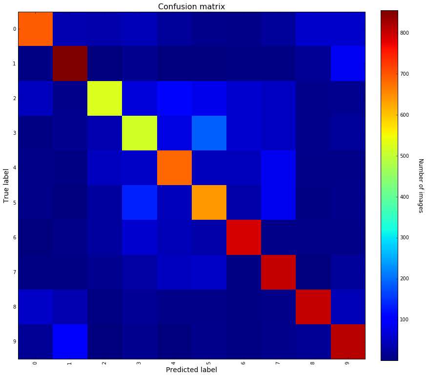
Knowing the class labels : 0 : airplane 1 : automobile 2 : bird 3 : cat 4 : deer 5 : dog 6 : frog 7 : horse 8 : ship 9 : truck
One can notice that the classes for which the F1-score is below 70% all correspond to animals.
Some remarkable facts out of the confusion matrix :
With minimal efforts, we managed to reach an average F1-score of 71%, which is not that bad for a classification task with 10 labels. To improve the performances (the Kaggle leaderboard demonstrates that the mean accuracy can go up to 95%), we could set up more complex model architectures so as to refine the feature extraction. It could also be worth trying some pre-processing on the images, for example finding a way to handle the blue-sky backgrounds that are misleading the classification for planes and birds.