-
Kernix Lab,
-
Data scientist
Publié le 07/11/2016
With the democratization of the internet, interacting and sharing knowledge is simpler than ever. This digital world has enabled a whole new way of consuming, learning, communicating and creating relationships, unleashing an enormous amount of data that we can analyze to get a better understanding of human behavior.
One way that we can use this data is to build networks of relationships between individuals or objects (friendships between Facebook users, co-purchasing of products on Amazon, genetic co-occurrence etc…). The field of community detection aims to identify highly connected groups of individuals or objects inside these networks, these groups are called communities.
The motives behind community detection are diverse: it can help a brand understand the different groups of opinion toward its products, target certain groups of people or identify influencers, it can also help an e-commerce website build a recommendation system based on co-purchasing, the examples are numerous. If you want to learn about community detection in more detail, you can read about it here.
The aim of this article is to introduce you with the principal algorithms for community detection and discuss how we can evaluate their performance to build a benchmark. Furthermore, depending on the field we are studying, we encounter many different types of networks and this can cause variations in the algorithms’ performance. That’s why we will also try to understand what elements of a network’s structure affect the performance of these algorithms.
Different methods have emerged over the years to efficiently uncover communities in complex networks. The most famous principle is maximizing a measure called modularity in the network, which is approximately equivalent to maximizing the number of edges (relationships) inside the communities and minimizing the number of edges between the communities. The first greedy (in terms of computation) algorithm based on modularity was introduced by Newman in 2004. He was already at the origin of the Girvan-Newman algorithm in 2002 which consists in progressively removing edges with high betweenness (likely to be between communities) from the network. Another method to detect communities is by simulating random walks inside the network. It is based on the principle that a random walker will tend to stay inside densely connected areas of the graph. That is the idea behind the walktrap algorithm, introduced by Pascal Pons and Matthieu Latapy in 2005. It also inspired the infomap algorithm created in 2008 by Martin Rosvall.
However, these algorithms only consider one community per node, which might be a wrong hypothesis in some cases. Several papers on the subject base their models on overlapping communities (i.e. where nodes can belong to several communities). The clique percolation method, made popular by Cfinder (freeware for overlapping community detection) in 2005, is the most recognized method to detect overlapping communities. The concept is that a network is made of many cliques (subsets of nodes such that every two distinct nodes in the clique are adjacent) which overlap. One clique can thus belong to several communities. Jaewon Yang and Jure Leskovec also published a paper in 2013 for their own overlapping community detection algorithm called BigClam. The particularity of this algorithm is that it is very scalable (unlike the algorithms mentioned before) thanks to non-negative matrix factorization. The authors claim that contrary to common hypothesis, community overlaps are denser than the communities themselves, and that the more communities two nodes share, the more likely they are to be connected. You can find here and here reviews of these different methods.
The issue at hand is to determine which algorithm we should use if we want to detect communities in a network. Is there one « best » algorithm? Or does it depend on the network we are studying and the aim of our study? First, we have to establish the criteria we want to compare the algorithms on. The most efficient way of evaluating a partition is to compare it to the communities we know exist in our network, they are called « ground-truth » communities. Several measures enable us to make that comparison, notably the normalized mutual information (NMI) and the F-Score.
There are two famous benchmark networks generators for community detection algorithms: Girvan-Newman (GN) and Lancichinetti-Fortunato-Radicchi (LFR). Since it is difficult to obtain many instances of real networks whose communities are known, a solution is to generate networks with a built-in community structure. It is then possible to evaluate the performance of the algorithms (usually with the NMI). The most famous and basic generator (GN) was not acknowledged as a realistic option. Indeed, the networks generated are not representative of the heterogeneity found in real-life networks (in particular, all the nodes have approximately the same degree when a « real » network should have a skewed degree distribution). A more realistic benchmark was then introduced (LFR), where the node degrees and community sizes are distributed according to power law.
You can read about these benchmarks algorithms here and here. However, the LFR benchmark doesn’t consider overlapping communities and generating large graphs could take some time depending on your computation capacities. This is why we are going to use real-life networks available on the Stanford large network dataset collection to build our benchmark. There are five networks
with ground-truth communities (Amazon, DBLP, Orkut, Youtube and Friendster) but we won’t be able to use the Friendster graph because of its volume. To manipulate the data and the algorithms, we will use the python igraph library.
Let’s load the Amazon graph and try the fastgreedy community detection algorithm. In this graph, the nodes are products and a link is formed between two products if they are often co-purchased.
For this algorithm, the graph needs to be undirected (no direction for the edges). It should take just under 15 minutes to get a result. As you can see, you get a list of the nodes’ community ids.
import igraph as ig
g = ig.Graph.Read_Ncol('/Users/Lab/Documents/DonneesAmazon/com-amazon.ungraph.txt')
print 'number of nodes: '+ str(len(g.vs()))
print 'number of edges: '+ str(len(g.es()))
Applying the fastgreedy algorithm
g=g.as_undirected()
dendrogram=g.community_fastgreedy()
clustering=dendrogram.as_clustering()
membership=clustering.membership
print membership[0:30]
Now that you have a membership list for the nodes, how can you quantitatively evaluate the quality of the partition made by the algorithm (you could want to evaluate it visually but this network is way too big) ? As we said before, the best way to do that is to compare our membership list to the ground-truth membership list via a performance measure. There are functions implemented in scikit-learn for this task but the issue is that these functions only consider non-overlapping communities whereas the ground-truth communities of our graphs are overlapping. This means we have to create a performance measure that takes into account overlapping communities. Luckily, Yang and Leskovec’s article on BigClam puts forward its own benchmark based on the datasets we are using. We decided to implement their performance method, which computes the F-Score on subgraphs of the original graph. This method solves the problem of the overlapping communities since we implement the F-Score ourselves, but it also solves the scalability problem of some algorithms which can’t work on our biggest graphs.
The F-score is the harmonic mean of precision and recall. More precisely, precision is the number of true positives divided by the total number of positives (among the nodes I have classified in a community, how many actually belong to that community ?), and recall is the number of true positives divided by the number of true positives and false negatives (how many nodes did I correctly classify in one community in comparison to the total number of nodes in that community ?).
Let’s break down the performance evaluation method (see Stanford’s article for more details and here for the whole PerformanceFScore script):
The first step is to randomly select a subgraph inside our original graph (a subgraph is made of at least two ground-truth communities).
Selection of a sugbraph
#Here, we randomly select a node in our network to build a subgraph around it.
Com=[0] #Number of communities of the node.
#A node must have at least two communities.
while len(Com)<2:
    #A node is selected randomly.
    rand=randint(0,len(g.vs()))
    node=g.vs[rand]
    #We check if the node was classified in a  community (if he exists in the ground-truth file).
    if node["name"] in nbComPerNode.keys():
        #We get the communities he belongs to.
        Com=nbComPerNode[node["name"]]

    else:
        continue
#In the ground-truth file, we take all the nodes that share at least one community with our original node.
GT={}
with open(FileGT,"r") as filee:
    for indx,line in enumerate(filee):
        if indx in Com:
            line = line.rstrip()
            fields = line.split("\t")
            nodes=[]
            for col in fields:
                nodes.append(col)
            GT[indx]=nodes
filee.close()

#We transform the node names into node indices to create the subgraph with igraph.
ndsSG=set()
for com in Com:
    temp=[nomIndice[k] for k in GT[com]]
    ndsSG.update(temp)
    ndsSG.add(node.index)

subgraph=g.subgraph(ndsSG)
We apply the community detection algorithm of our choice on the subgraph.
#We apply the algorithm.
commClus=ChoixAlgo(algo,subgraph,commClus,path,SnapPath)
We compute the F-Score between all detected communities and all ground-truth communities and keep the highest (we do that as many times as there are detected communities and take the mean of the highest F-Scores). We compute the F-Score between all ground-truth communities and detected communities and keep the highest (we do that as many times as there are ground-truth communities and take the mean of the highest F-Scores).
Computation of the F-Score
def calculFScore(i,j):
    i=[int(x) for x in i]
    j=[int(x) for x in j]
    inter=set(i).intersection(set(j))
    precision=len(inter)/float(len(j))
    recall=len(inter)/float(len(i))
    if recall==0 and precision==0:
        fscore=0
    else:
        fscore=2*(precision*recall)/(precision+recall)
    return fscore
We take the mean of the two mean F-Scores.
#This gives the F-Score on one subgraph
measure=(fscore1+fscore2)/2
We repeat the operation on another subgraph.
In the end, we take the mean of the F-Scores on all the subgraphs. However, the F-Score that you get should be really low, which is why we normalize the scores between 0 and 1. We selected five algorithms to compare here : snap’s infomap, igraph’s infomap, igraph’s fastgreedy, snap’s cpm and snap’s BigClam. This way we can compare the most popular algorithms for non-overlapping communities with algorithms for overlapping communities.
For all of our graphs we get the same ranking. Igraph’s infomap gets the best F-Score, closely followed by snap’s infomap. Then we have in this order and close : BigClam, cpm and fastgreedy. However, we have to keep in mind that the F-Score favors big communities and that infomap tends to create big communities.
Here is an example of the ranking we get on the Amazon graph : 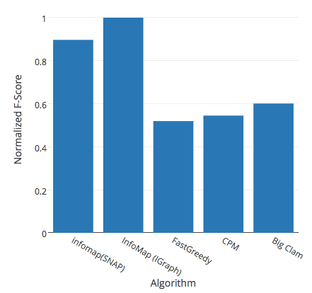
This result is surprising since we have some graphs with a lot of overlaps (like the Amazon graph which has an overlap rate of 0.95) but the overlapping community detection algorithms don’t work better on it than on the DBLP graph which has an overlapping rate of 0.35. As a reminder, in the DBLP graph the nodes are authors of research papers in computer science, and two authors are linked if they wrote at least one paper together. It means that even if a graph has indeed a lot of overlapping communities, the dedicated algorithms are not able to correctly identify these overlaps enough to have a better performance than infomap (at least on our test graphs). However, it is acknowledged that the various types and structures of graphs in real life affect the results of the algorithms. Indeed, the algorithm we want to use has to be adapted to the structure of our graph.
Depending on the field or the context we are studying, we can encounter many different structures in graphs. if we take subgraphs of the Youtube and DBLP graphs, we can tell that their structures are quite different :
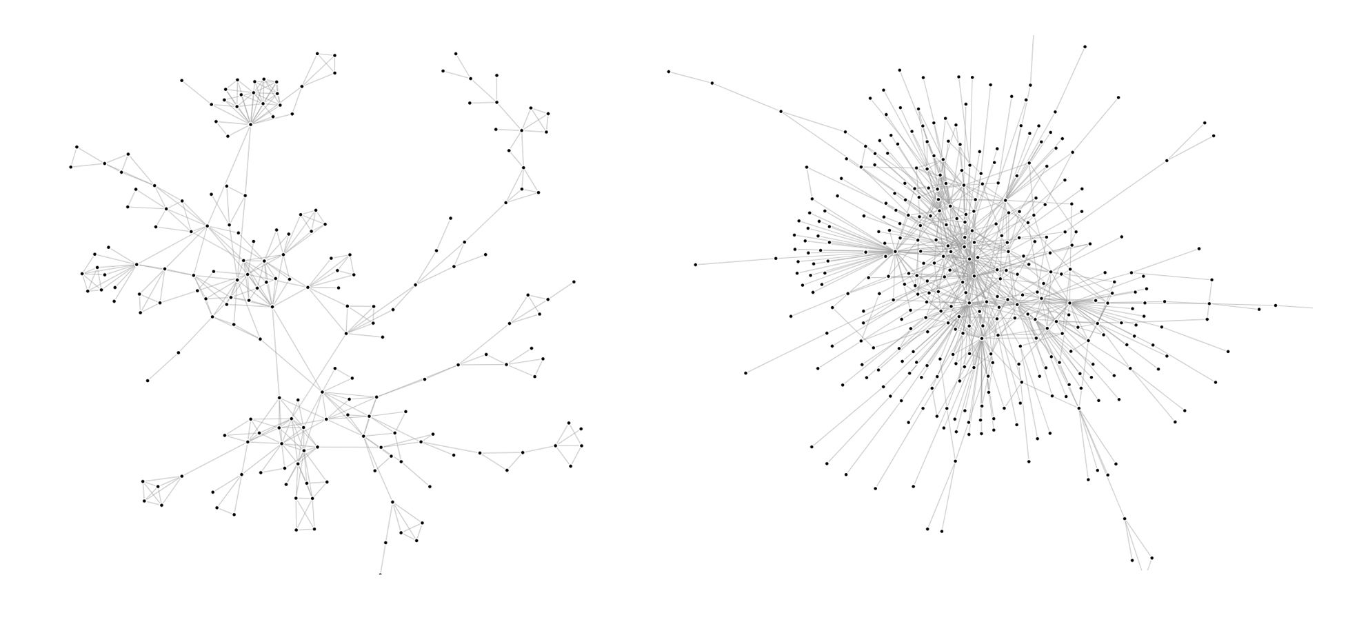
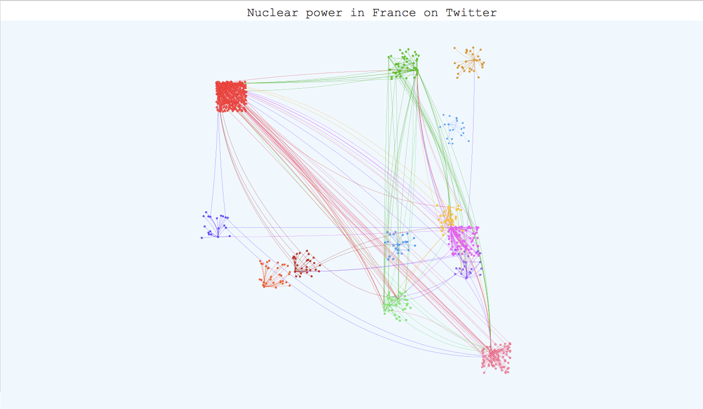
Indeed, the Youtube subgraph has a clear tree structure whereas the DBLP subgraph has more of a wheel structure. What is the impact of one structure or the other on the algorithms’ performance? To understand that, we created a small graph from twitter data on the subject of nuclear power (The snap graphs are too big to easily apply our algorithms and create visualizations). The nodes (998 in total) are users and the edges are retweets. The structure is identical to the Youtube subgraph’s (tree). Let’s visualize the results of different
community detection algorithms on this graph :
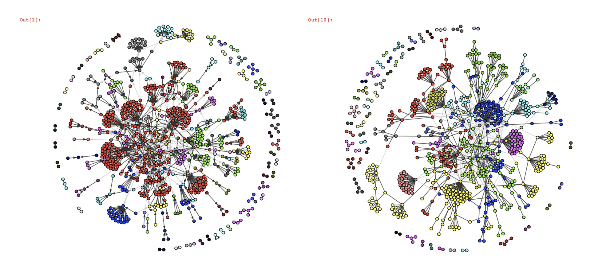
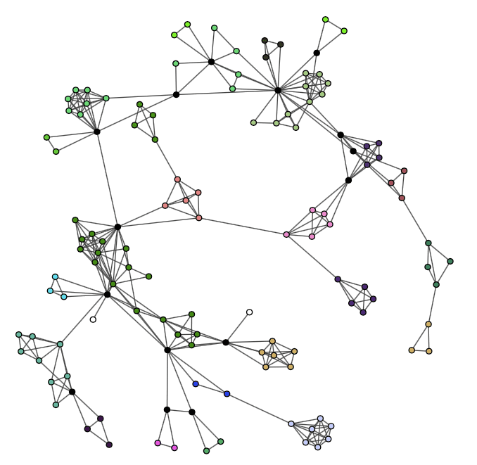
Judging only by the visualizations since we don’t have the ground-truth communities, Infomap and fastgreedy seem to work well on this graph structure, the only difference is that whereas infomap creates one big community (in red), fastgreedy tends to break it in little communities. However, as the graph grows in size, the algorithms’ behaviour reverse and fastgreedy struggles more and more to detect smaller communities whereas infomap becomes a lot more precise.
Here, which algorithm to use depends on the aim of your study : in the long term, fastgreedy won’t be very good at detecting small communities and will tend to merge them together (this is called the resolution limit), but you might want bigger, more global communities. Infomap is better at identifying smaller groups of people who follow one particular leader, so it’s the way to go if you want a precise community detection (which is usually better). A final vizualisation of the result for infomap in javascript is available later in the article, there were too many nodes to simply process with matplotlib.
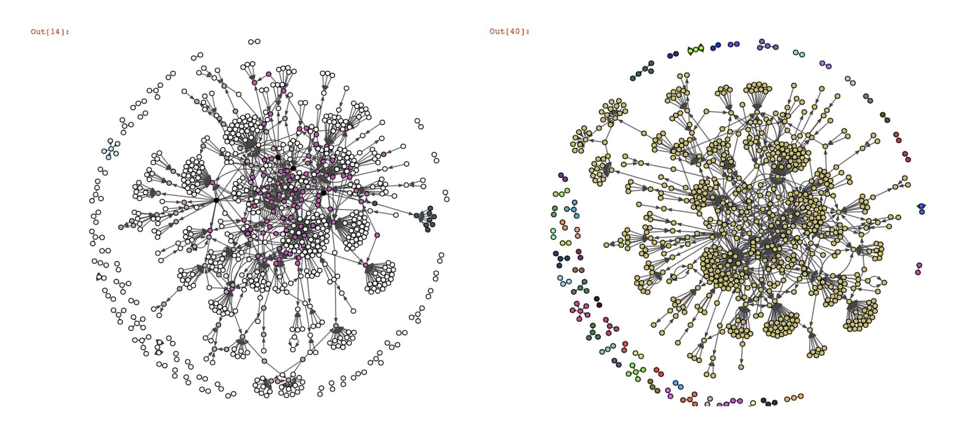
On the contrary, we can see that the overlapping community detection algorithms BigClam and cpm don’t work at all on our twitter graph. Most of the nodes are not classified (nodes in white, the black nodes belong to several communities). The reason for that is the way these algorithms detect the communities.
The cpm (clique percolation) algorithm tries to find cliques inside the graph (the number of nodes per clique k is a parameter of the algorithm). The issue with this graph is that there are no cliques made of more than two nodes and there are very little possibilities of overlap between the cliques, which makes it very difficult for the algorithm to identify them (even more if k>2). We also tried the kclique algorithm from the networkx library (which is based on the clique percolation method), but with k=2 the algorithm classifies almost all the nodes in one community and with k>2, it gives the same kind of result as cpm. The BigClam algorithm tries to find overlaps between communities initiated with locally minimal neighborhoods, but given the structure of our graph, these initialization communities should have very little overlap.
The twitter graph is a good example of a structure that is not suited for these overlapping community detection algorithms. A solution to that would be to change the way we select our twitter data to get a more appropriate structure. For example, we could consider studying the replies or the mentions between users. Let’s take a subgraph of our DBLP test graph, where the structure is very different from the twitter graph, and observe the result of the cpm algorithm:
This result shows that the clique percolation method works way better on a wheel structure, where overlaps are more likely and more easily identifiable. However, infomap still had a better performance overall in the sense of the F-Score on this graph. Infomap and fastgreedy also seem to work pretty well on the twitter graph so we could just use those instead of overlapping algorithms.
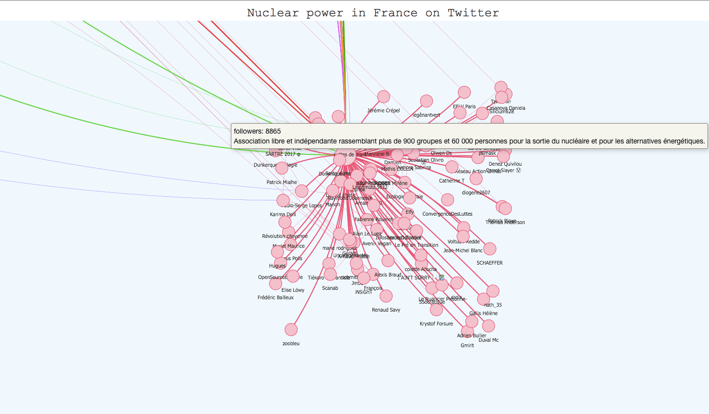
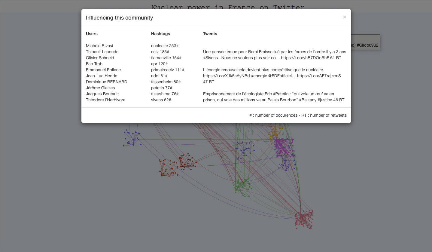
Once you have applied your community detection algorithm on your graph and you are satisfied with the result, it can be very interesting to build an interactive visualization. It helps materialize your community detection and get a global point of view on your communities and their members. The igraph library has a plot function for this task but the visualization is not interactive. However, there are differents javascript libraries that offer very interesting interactive templates. D3.js has a force-layout graph template where you can play with the nodes and move them around, but Vis.js has a very complete template for community detection visualization that we tried with our twitter graph. All we had to do was adapt our data to the template (it takes json or js files) and use boostrap.js to add descriptions for the communities. The visualization is available on the kernix github here , and the original template here. Here are several screenshots :
To conclude this post, community detection in complex networks is still a very challenging field. Many algorithms have been created to efficiently identify communities inside large networks, infomap being recognized as the most reliable. However, correctly evaluating the performance of these algorithms is still an issue, especially in the case of overlapping communities. The only way we can appreciate the quality of an algorithm is to test it on a graph with a built-in community structure, or where we know the ground-truth communities, and even then, there isn’t any implemented measure for overlapping communities. Maybe completing community detection on large graphs with semantical analysis could be a way to have a little more control on the results.
We still saw with the example of the twitter graph that some algorithms yield pretty good results on small graphs (given that we use the best suited algorithms for the graph’s structure), and in this case the graph is small enough to build a nice visualization of our result and get an idea of the quality of the partition.
