-
Kernix Lab,
-
Data scientist
Publié le 06/05/2016
Further to our previous tutorial « An efficient recommender system based on graph database« , hereafter is another method to implement a movies recommender system based on movies synopses. The principle is to use movie synopses to automatically identify other movies similar to the ones the user likes. How? by using natural language processing.
This recommender system is built on an item-based method, also called content-based method, for which the similarity between items (in our case, movies) is exploited. The recommender system identifies movies that the user has highly rated in the past, and then suggests movies very similar to its tastes and preferences.
In order to build such a recommender system, we have to answer the questions: how do we get movies synopses? how do we measure the similarity between movies based on their synopsis? how do we add this new relationship to the Neo4j graph? and how do we exploit it to produce a list of recommendation for a given user? In the following, we explain the method and answer to all of these questions.
The MovieLens 100k dataset, fully described in the previous tutorial, contains an IMDb URL field allowing a direct access to the IMDb page of a movie to retrieve its synopsis. However, this URL is not always reliable: it can redirect us to a search page with several movies results or can even be unknown. In addition, some movies don’t have a synopsis but a short description and/or a story line. Also, it is important to note that the synopsis is not included in the movie page, but is available through a link to another page.
In the following, we present a python code addressing these limitations. We use the lxml library to get the html content of a page, and the IMDb library to get the IMDb information based on the movie IMDb id. Using the following code, we successfully retrieved the summary of 1021 movies out of 1661. To load the movie DSV file (u.item) refer to the third code cell of the previous tutorial.
# from imdb import IMDb
ia = IMDb()
from lxml import html
import requests
#
movie['synopsis'] = ''
movie['storyline'] = ''
movie['description']= ''
movie['text'] = ''
# Looping over movies
for index, row in movie.iterrows():
    if (row['IMDb url'] != 'unknown'):
        # Get the html content
        page = requests.get(row['IMDb url'])
        tree = html.fromstring(page.content)
        try:
            # Get the movie id
            idm = tree.xpath('/html/head/meta[6]')[0].get('content')[2:]
            # Get the story line
            movie.loc[index, 'storyline'] = tree.xpath('//*[@id="titleStoryLine"]/div[1]/p/text()')[0]
            # Get the movie using the IMDB library based on the movie id
            m = ia.get_movie(idm)
            # Get the descreption
            movie.loc[index, 'description'] = m.get('plot outline')
            # Get the synopsis
            ia.update(m, 'synopsis')
            if m.get('synopsis') is not None:
                movie.loc[index, 'synopsis'] = m.get('synopsis')
        except IndexError:
            pass
    # Create a text field to concatenate all existing summaries
    movie.loc[index, 'text'] = movie.loc[index, 'description'] + ' ' + movie.loc[index, 'storyline'] + ' '+ movie.loc[index, 'synopsis']
When the URL doesn’t redirect to the right page, we can use the IMDb library to get information about a movie based on its title using the search_movie(title) function. However, this function is a simple search action which returns a list of movies sorted by relevance. In the following code, we ensure that the first element of the search list is the expected movie title. We then get its description and synopsis using its IMDb id.
import collections
compare = lambda x, y: collections.Counter(x) == collections.Counter(y)
for index, row in movie.iterrows():
    if row.text.strip() == '':
        title = row.title
        title = title.replace('(', '')
        title = title.replace(')', '')
        title = title.replace(',', '')
        ia = IMDb('http')
        m = ia.search_movie(row.title)
        if len(m) !=0:
            m = m[0]
            try:
                title_found = m['title']+ ' ' +str(m['year'])
                if compare(title.split(), title_found.split()):
                    m = ia.get_movie(m.movieID)
                    movie.loc[index, 'description'] = m.get('plot outline')
                    ia.update(m, 'synopsis')
                    movie.loc[index, 'synopsis'] = m.get('synopsis')
                    movie.loc[index, 'text'] = movie.loc[index, 'description'] + ' ' + movie.loc[index, 'synopsis']
            except:
                pass
Using this code, we successfully retrieve the summary of 345 additional movies. As a result, we retrieve summaries for 1366 movies in total, out of 1661. In the next section, we show how these synopses can be used to establish a similarity relationship between movies.
To identify the similarity between movies based on their synopsis, we use the « latent semantic analysis » (LSA) which is a widely used technique in natural language processing. LSA transforms each synopsis into a vector in a space of features. In our case, the features are words occuring in the synopses. Then, a matrix containing all vectors is created: columns represent the synopses of movies and rows represent unique words. Accordingly, the number of rows can amount to tens of thousands of words. In order to identify the relevant features of this matrix, the « singular value decomposition » (SVD), which is a popular dimension reduction technique, is used to reduce the number of rows -words- while maintaining and highlighting the similarity between columns -synopses-. The dimension of this approximation matrix is set by a hyper-parameter which is the number of topics. In this framework, a topic consists of a set of words with associated weights defining the contribution of each word to the direction of this topic. Based on this low-dimensional approximation matrix, the similarity between two columns -synopses- is calculated using the cosine of the angle between these two vectors.
Hereafter we detail all steps to create a LSA model and compute the similarity between synopses. Here are the mains steps:
1- Pre-processing the synopses: First of all, we remove punctuations and irrelevant words like stop words and persons’ names. This will avoid topics in which these words represent the keywords (for instance, « however », « michael », « none » and « laura » will not define a topic).
In addition, we use the Snowball stemmer, also called Porter2 stemmer, to detect similar words present in different formats (remove suffix, prefix, etc.). Snowball is a language, developed by M.F. Porter, to efficiently define stemmers (see Snowball: A language for stemming algorithms for more information). This stemming algorithm is the most used one in the natural language processing domain.
The Natural Language Toolkit (nltk) provides a large number of methods covering different topics in the human language data domain, like classification, stemming, tagging, parsing and semantic reasoning.
## Remove punctuations
from nltk.tokenize import RegexpTokenizer
tokenizer = RegexpTokenizer(r'\w+')
movie['text'] = movie['text'].apply(lambda x: ' '.join(tokenizer.tokenize(x)))
documents = list(movie['text'])
from nltk.corpus import stopwords
stop_words = set(stopwords.words('english'))
## Extract the persons' names
import nltk
def extract_entities(name, text):
    # Lopping over the sentences of the text
    for sent in nltk.sent_tokenize(text):
        # nltk.word_tokeize returns a list of words composing a sentence
        # nltk.pos_tag returns the position tag of words in the sentence
        # nltk.ne_chunk returns a label to each word based on this position tag when possible
        for chunk in nltk.ne_chunk(nltk.pos_tag(nltk.word_tokenize(sent))):
            try:
                if chunk.label() == 'PERSON':
                    for c in chunk.leaves():
                        if str(c[0].lower()) not in name:
                            name.append(str(c[0]).lower())
            except AttributeError:
                pass
    return name
##
names = []
for doc in documents:
    names = extract_entities(names, doc)
## Update the stop words list
stop_words.update(names)
## Remove stop words and persons names and Get word stem
from nltk.stem import SnowballStemmer
stemmer = SnowballStemmer("english") # Choose a language

texts = [[stemmer.stem(word) for word in document.lower().split() if (word not in stop_words)]
          for document in documents]
2- Creating the dictionary: The dictionary consists of a concatenation of unique words of all synopses. Gensim is an efficient library to analyse the latent semantic similarity between documents.
from gensim import corpora, models, similarities
dictionary = corpora.Dictionary(texts)
This function maps unique words with their ids. In our case, the length of the dictionary is equal to 15035 words which means that each synopsis will be represented through a 15035-dimensional vector space.
list(itertools.islice(dictionary.token2id.items(), 0, 20))
3- Creating the corpus: The corpus is the collection of all synopses pre-processed and transformed using the dictionary.
corpus = [dictionary.doc2bow(text) for text in texts]
Accordingly, the corpus object contains the movies synopses, represented as sparse vectors. Here is the example of the fourth movie synopsis.
print(corpus[3][:20])
The vector feature (48, 1.0) means that the word with id=48 (‘name’) appears once in the entire corpus[3] (fourth movie synopsis).
dictionary[48]
4- Creating the tf-idf transformation: The term frequency-inverse document frequency (tf-idf) transformation reflects the importance of words in the corpus. The (tf-idf) value of a word depends not only on the word count in a document, but also on the number of occurrences in the corpus.
To explain the principle of this transformation, let us consider emphasizing movies relating to « the artificial intelligence ». A straightforward method would consist in counting the occurrences of each of these three terms (« the », « artificial », « intelligence ») in movies synopses and computing the similarity based on their « term frequency ». The problem of such a method is that the term « the » is a very common word. The associated term frequency will tend to select movies in which the term « the » is used more frequently. The idea of « inverse document frequency » is to give a relevance weight to different terms. Accordingly, the idf associates a low weight to terms that appear frequently in the corpus and increases the weight of terms that rarely appear.
tfidf = models.TfidfModel(corpus)
corpus_tfidf = tfidf[corpus]
The « tfidf » function transforms the corpus from a bag-of-words integer counts representation into tf-idf real values weight.
print(corpus_tfidf[3][:20])
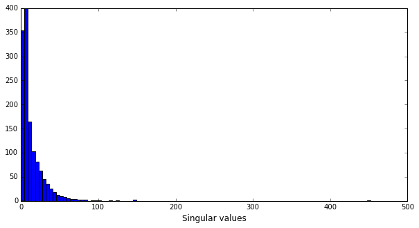
5- Choice of the number of topics: As mentioned above, LSA seeks to identify a set of topics related to the movies synopses. The number of these topics N is equal to the dimension of the approximation matrix resulting from the SVD dimension reduction technique. This number is a hyper-parameter to be carefully adjusted. It results from the selection of the N largest singular values of the tf-idf corpus matrix. These singular values can be calculated as follows:
numpy_matrix = gensim.matutils.corpus2dense(corpus, num_terms=51556)
s = np.linalg.svd(numpy_matrix, full_matrices=False, compute_uv=False)
A histogram of the singular values of the tf-idf corpus matrix is presented in the following figure.
plt.figure(figsize=(10,5))
plt.hist(s[0], bins=100)
plt.xlabel('Singular values', fontsize=12)
plt.show()
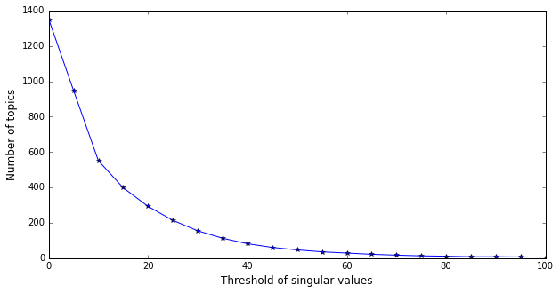
We then set several thresholds for the singular values and we compute the relative number of topics. We can see that from threshold equals 60, the number of topics is stabilized to 30 topics (figure bellow). This choice appears to be logical as the number of movie genres in this database is equal to 19.
plt.figure(figsize=(10,5))
plt.plot(range(0,101,5), nbr, '*-')
plt.xlabel('Threshold of singular values', fontsize=12)
plt.ylabel('Number of topics', fontsize=12)
6- Creating the LSA model:
lsi = models.LsiModel(corpus_tfidf, id2word=dictionary, num_topics=30)
The « LsiModel » function transforms our tf-idf corpus into a latent 30-dimensional space (number of topics = 30).
index = similarities.MatrixSimilarity(lsi[corpus_tfidf]) # transform corpus to LSI space and index it
7- Computation of the similarity between synopses:
movie['similarity'] = 'unknown'
movie['size_similar'] = 0
total_sims = [] # storage of all similarity vectors to analysis
thershold = 0.2
for i, doc in enumerate(corpus_tfidf):
    vec_lsi = lsi[doc] # convert the vector to LSI space
    sims = index[vec_lsi] # perform a similarity vector against the corpus
    total_sims = np.concatenate([total_sims, sims])
    similarity = [] # Create a list with movie_id and similarity value
    for j, x in enumerate(movie.id):
        if sims[j] > thershold:
            similarity.append((x, sims[j]))
    similarity = sorted(similarity, key=lambda item: -item[1])
    movie = movie.set_value(i,'similarity', similarity)
    movie = movie.set_value(i,'size_similar', len(similarity))
db_similarity = movie[['id', 'similarity']]
db_similarity.to_csv('./ml-100k/u.similarity', sep='|') # store the similarity results
Now, we will introduce a new relationship between two movies based on the semantic similarity computed between their synopses. These similarity relationships can be easily added to the Neo4j graph as shown in the previous tutorial.
from ast import literal_eval
# Loading similarity data
similarity_db = pd.read_csv('ml-100k/u.similarity', sep='|')
# Create "Similarity" relationship between the similar movies with score equal to the rate of similarity
tx = graph.cypher.begin()
statement = ("MATCH (m_ref:Movie {movie_id:{A}}) "
             "MATCH (m:Movie {movie_id:{B}}) MERGE (m_ref)-[r:`Similarity` {score: {C}}]->(m)")

# Looping over movies m
for index, m in similarity_db.iterrows() :
    # Trasform the m.similarity into a list
    similarity = literal_eval(m.similarity)
    # Looping over movies similar to m
    for sim in similarity:
        if sim[0] != m['id']:
            tx.append(statement, {"A": m['id'], "B": sim[0], "C": sim[1]})
    tx.process()
    if index%10==0 :
        tx.commit()
        tx = graph.cypher.begin()

tx.commit()
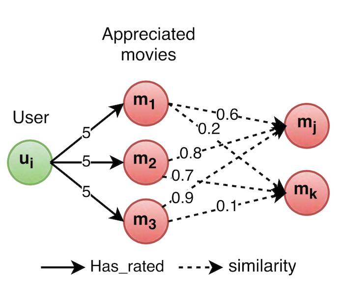
Hereafter, we show how the semantic similarity between movies can be used to perform recommendations. Quite simply: for a given user, we identify the movies that were appreciated (for example, rated more than 4) and then we recommend movies similar to the appreciated ones (for example, similarity score more than 0.7). You are probably wondering how we manage a movie which is similar to several appreciated ones. Well, we simply compute the sum of the relative similarity scores to emphasize movies similar to several appreciated ones (cf. following figure).
Accordingly, for a given user, the recommendation is performed in three steps:
As in the previous tutorial, for each of these methods we asked our guinea pig to attribute ratings to the top 20 suggested movies in order to evaluate the performance of recommendations.
The above recommendation description can be formulated by the following py2neo/Cypher query:
query = ('MATCH (user:User {user_id:{user_id}}) ' # Identify the user based on its id
         # Identify the unwatched movies (when no ":Has_rated" relationship between the user and the movie
        'MATCH (unwatched:Movie) '
        'WHERE NOT ((user)-[:Has_rated]->(unwatched)) '
         # Store the ids of the unwatched movies into a set
        'WITH collect(unwatched.movie_id) as unwatched_set, user '
        'MATCH (user)-[rate:Has_rated]->(appreciated:Movie) '
        'WHERE rate.rating > {threshold_appreciated} '
         # Identify unwatched movies similar to the appreciated movies
        'MATCH (appreciated)-[sim:Similarity]-(reco:Movie) '
        'WHERE reco.movie_id in unwatched_set and sim.score > {threshold_similar} '
         # Return the recommentations based on the sum of similarity scores
        'RETURN distinct reco.movie_id as movie_id, reco.title, sum(sim.score) as score '
        'ORDER BY score DESC')
tx = graph.cypher.begin()
tx.append(query, {"user_id":user_id, "threshold_appreciated":threshold_appreciated, "threshold_similar":threshold_similar})
result = tx.commit()
The following table presents the top 20 suggestions with the ratings attributed by our guinea pig.
| Movie Title | Rating | |
|---|---|---|
| 1 | Phantoms (1998) | – |
| 2 | The Crow (1994) | – |
| 3 | Mimic (1997) | – |
| 4 | The Hunchback of Notre Dame (1996) | 4 |
| 5 | A Nightmare on Elm Street (1984) | – |
| 6 | The Howling (1981) | – |
| 7 | Vertigo (1958) | 5 |
| 8 | Highlander (1986) | 1 |
| 9 | Indiana Jones and the Last Crusade (1989) | 5 |
| 10 | Batman (1989) | 5 |
| 11 | Hercules (1997) | 3 |
| 12 | The Outlaw (1943) | – |
| 13 | Beauty and the Beast (1991) | 5 |
| 14 | Nosferatu (1922) | 5 |
| 15 | The Truman Show (1998) | 5 |
| 16 | Lost World: The Jurassic Park (1997) | 4 |
| 17 | Contact (1997) | 4 |
| 18 | The Amityville Horror (1979) | – |
| 19 | Dracula: Dead and Loving It (1995) | 2 |
| 20 | Alphaville (1965) | – |
Here, our guinea pig provides ratings to 12 movies out of 20 which means that he has watched these movies. Two movies that don’t match his tastes are proposed. However, « Dracula: Dead and Loving It » is not a popular movie (average rating equal to 2.8). Accordingly, this recommendation strategy can be slightly modified to take into account the global rating (average of all users’ rating) associated to the recommended movies. In other words, we recommend movies similar to those appreciated by the user, and we sort this list of recommendations by the sum of similarity scores of a movie weighted by its global rating.
In what follows, the py2neo/Cypher query corresponding to these modifications.
query = ('MATCH (user:User {user_id:{user_id}}) ' # Identify the user based on its id
         # Identify the unwatched movies (when no ":Has_rated" relationship between the user and the movie
        'MATCH (unwatched:Movie) '
        'WHERE NOT ((user)-[:Has_rated]->(unwatched)) '
         # Store the ids of the unwatched movies into a set
        'WITH collect(unwatched.movie_id) as unwatched_set, user '
        'MATCH (user)-[rate:Has_rated]->(appreciated:Movie) '
        'WHERE rate.rating > {threshold_appreciated} '
         # Identify unwatched movies similar to the appreciated movies
        'MATCH (appreciated)-[sim:Similarity]-(reco:Movie) '
        'WHERE reco.movie_id in unwatched_set and sim.score > {threshold_similar} '
        'WITH collect(reco.movie_id) as reco_set, user, sim, reco '
         # Global ratings of the recommended movies
        'MATCH (users:User)-[r:Has_rated]->(m:Movie) '
        'Where m.movie_id in reco_set '
         # Return the recommentations ordered on the sum of similarity scores weighted by the global rating
        'RETURN distinct reco.movie_id as movie_id, reco.title, sum(sim.score)*avg(r.rating) as score '
        'ORDER BY score DESC')
tx = graph.cypher.begin()
tx.append(query, {"user_id":user_id, "threshold_appreciated":threshold_appreciated, "threshold_similar":threshold_similar})
result = tx.commit()
The following table presents the top 20 suggestions with the ratings attributed by our guinea pig.
| Movie Title | Rating | |
|---|---|---|
| 1 | Contact (1997) | 4 |
| 2 | Indiana Jones and the Last Crusade (1989) | 5 |
| 3 | The Princess Bride (1987) | – |
| 4 | L.A. Confidential (1997) | – |
| 5 | Vertigo (1958) | 5 |
| 6 | Men in Black (1997) | 4 |
| 7 | Star Trek: First Contact (1996) | Not interessed |
| 8 | Beauty and the Beast (1991) | 5 |
| 9 | It’s a Wonderful Life (1946) | – |
| 10 | Batman (1989) | 5 |
| 11 | Lawrence of Arabia (1962) | 5 |
| 12 | M*A*S*H (1970) | 5 |
| 13 | Highlander (1986) | 1 |
| 14 | Psycho (1960) | 5 |
| 15 | Stand by Me (1986) | – |
| 16 | The Hunt for Red October (1990) | 4 |
| 17 | Mars Attacks! (1996) | 5 |
| 18 | Liar Liar (1997) | 3 |
| 19 | The Crow (1994) | – |
| 20 | Face/Off (1997) | 4 |
The introduction of the movies rating has greatly improved the recommendation performance. Despite « Highlander », all the already watched movies match the tastes of our guinea pig. Accordingly, we could hope that he will also appreciate the unwatched ones. The reason for which « Highlander » remains in the list of recommendations is that this movie is similar to highly appreciated movies and its average rating (3.5) is relatively good.
This tutorial confirms the conclusions of the previous one. The item-based method presented in this tutorial and the user-based one are two complementary strategies. In most cases, these two methods produce different suggested movies which address different aspects of user’s tastes. Accordingly, the comparison of their respective results is not trivial. It relies on the purpose of the recommender system, and the establishment of specific criteria to evaluate its performance. This point is discussed in the previous tutorial. Nevertheless, providing the reason for which we suggest this or that movie may be convincing (« you have appreciated these movies, you may appreciate these ones », « what did similar users watch? »).In addition, the graph-based concept is very adapted to this problematic. The implementation of the graph is easy and fast. Creating 1661 movies, 944 users and all relationships between them can be achieved in less than two minutes. In almost five minutes, the synopses of the 1336 movies can be cleaned, the LSA model learned, the similarity between movies computed and the similarity relationship added to the graph. On top of that, providing a list of recommendations for a given user can be achieved in less than three seconds!The graph-based concept allows also a simple and easy-to-implement view of the different recommendation strategies. You have probably noticed that throughout these two tutorials we can imagine different modifications and this can be easily considered in the cypher query.
