- Stanislas Morbieu,
-
Data scientist
Publié le 26/09/2016
Textual data is ubiquitous. Computing semantic relationships between textual data enables to recommend articles or products related to a given query, to follow trends, to explore a specific subject in more details, etc.But texts can be very different miscellaneous: a Wikipedia article is long and well written, tweets are short and often not grammatically correct.
Word2vec, introduced in Distributed Representations of Words and Phrases and their Compositionality (Mikolov et al., NIPS 2013), has attracted a lot of attention in recent years due to its efficiency to produce relevant word embeddings (i.e. vector representations of words). Word2vec is a shallow neural network trained on a large text corpus. The meaning of a word is learned from its surrounding words in the sentences and encoded in a vector of real values. Explaining in more details how it is done is out of scope of this article, but the key points are that a precomputed model gives us real valued vectors associated to words and that those vectors contain a lot of information because the model is trained on a big dataset. A similarity measure between real valued vectors (like cosine or euclidean distance) can thus be used to measure how words are semantically related. As documents are composed of words, the similarity between words can be used to create a similarity measure between documents.
This is the topic of this article: we will show how to create similarity measures based on word2vec that will be particularly effective for short texts. Two short texts can be very similar while using different words, thus capturing the meaning of the words by word2vec and using this information to compare documents should allow us to find that similar documents using different words are indeed similar. This special case, where almost no overlapping exists between the words of the first document and those of the second, is not correctly handled with commonly used methods based on the Vector Space Model.
Two similarity measures based on word2vec (named « Centroids method » and « Word Mover’s Distance (WMD) » hereafter) will be studied and compared to the commonly used Latent Semantic Indexing (LSI), based on the Vector Space Model.
In order to compare the document similarity measures, we will use two datasets, 20 Newsgroups and web snippets. First we will collect them and preprocess them. Secondly, we will explain the similarity measures and build the associated models. Lastly we will compare them on a retrieval task: given a document, retrieve the most semantically related documents, and evaluate this on a more general task, a clustering task (i.e. group documents into semantic clusters). An overview of the methodology is given by the figure below (Figure 1):

In this part we will collect two datasets and preprocess them.
The two datasets are:
The two datasets differ a lot and this allows us to see in which conditions each model is better.
We first retrieve the ng20 dataset with scikit-learn library and preprocess it with nltk library to remove meaningless words (called stopwords). Each document is represented as a bag of words. The corpus is then a list of bag of words.
from sklearn.datasets import fetch_20newsgroups

from nltk import word_tokenize
from nltk import download
from nltk.corpus import stopwords

download('punkt')
download('stopwords')

stop_words = stopwords.words('english')

def preprocess(text):
   text = text.lower()
   doc = word_tokenize(text)
   doc = [word for word in doc if word not in stop_words]
   doc = [word for word in doc if word.isalpha()]
   return doc

# Fetch ng20 dataset
ng20 = fetch_20newsgroups(subset='train',
       remove=('headers', 'footers', 'quotes'))

# text and ground truth labels
texts, y = ng20.data, ng20.target

corpus = [preprocess(text) for text in texts]
Note that we removed the headers, footers and quotes as they give too much information about the relationship between mails.
In this corpus some documents are empty or meaningless, so we remove them as well:
def filter_docs(corpus, texts, labels, condition_on_doc):
    """
    Filter corpus, texts and labels given the function condition_on_doc which takes
    a doc.
    The document doc is kept if condition_on_doc(doc) is true.
    """
    number_of_docs = len(corpus)

    if texts is not None:
         texts = [text for (text, doc) in zip(texts, corpus)
                  if condition_on_doc(doc)]

         labels = [i for (i, doc) in zip(labels, corpus) if condition_on_doc(doc)]
         corpus = [doc for doc in corpus if condition_on_doc(doc)]

         print("{} docs removed".format(number_of_docs - len(corpus)))

         return (corpus, texts, labels)

corpus, texts, y = filter_docs(corpus, texts, y, lambda doc: (len(doc) != 0))
Note that we have defined a general function filter_docs because we will further filter our collection with different conditions later on.
Let’s introduce the other dataset.
The web snippets are available here: http://acube.di.unipi.it/tmn-dataset/.
In this dataset, a snippet is already a bag of words. This will not affect our study as we do not use the order of the words.
snippets = []
snippets_labels = []
snippets_file = "data/data-web-snippets/train.txt"
with open(snippets_file, 'r') as f:
    for line in f:
        # each line is a snippet: a bag of words separated by spaces and
        # the category
        line = line.split()
        category = line[-1]
        doc = line[:-1]
        snippets.append(doc)
        snippets_labels.append(category)

snippets, _, snippets_labels = filter_docs(snippets, None, snippets_labels,
                                           lambda doc: (len(doc) != 0))
Let’s now measure the semantic relationships of documents.
In this part, we will present three methods to compute document similarities.
LSI has been introduced in a previous post on natural language processing. This method relies on several steps:
We are using the gensim implementation of LSI, that needs a special representation for the corpus. We use the tf-idf weighting factor, construct our LSI model and compute the similarity between documents:
import numpy as np
from gensim import corpora
from gensim.models import TfidfModel
from gensim.models import LsiModel
from gensim.similarities import MatrixSimilarity

sims = {'ng20': {}, 'snippets': {}}
dictionary = corpora.Dictionary(corpus)
corpus_gensim = [dictionary.doc2bow(doc) for doc in corpus]
tfidf = TfidfModel(corpus_gensim)
corpus_tfidf = tfidf[corpus_gensim]
lsi = LsiModel(corpus_tfidf, id2word=dictionary, num_topics=200)
lsi_index = MatrixSimilarity(lsi[corpus_tfidf])
sims['ng20']['LSI'] = np.array([lsi_index[lsi[corpus_tfidf[i]]]
                                for i in range(len(corpus))])
The same steps are taken for the web snippets:
dictionary_snippets = corpora.Dictionary(snippets)
corpus_gensim_snippets = [dictionary_snippets.doc2bow(doc) for doc in snippets]
tfidf_snippets = TfidfModel(corpus_gensim_snippets)
corpus_tfidf_snippets = tfidf_snippets[corpus_gensim_snippets]
lsi_snippets = LsiModel(corpus_tfidf_snippets,
                        id2word=dictionary_snippets, num_topics=200)
lsi_index_snippets = MatrixSimilarity(lsi_snippets[corpus_tfidf_snippets])
sims['snippets']['LSI'] = np.array([lsi_index_snippets[lsi_snippets[corpus_tfidf_snippets[i]]]
                                    for i in range(len(snippets))])
The second method is based on word2vec, in order to exploit the information contained in word vectors. We first load a pre-trained word2vec model:
from gensim.models import Word2Vec

filename = 'GoogleNews-vectors-negative300.bin.gz'
word2vec_model = Word2Vec.load_word2vec_format(filename, binary=True)
We precompute the L2-normalized vectors and forget the original vectors (replace=True) to only keep the normalized ones. The normalization is useful to compute the euclidean distances between words. This is used both for this method when the mean of word vectors will be computed and for the third method (Word Mover’s Distance). Forgetting the original vectors saves memory and can only be used if we finished training the word2vec model.
word2vec_model.init_sims(replace=True)
A simple method to exploit words representations for document representation and similarity is to compute for a given document, the mean of its words vectors. An illustration is given in Figure 2:
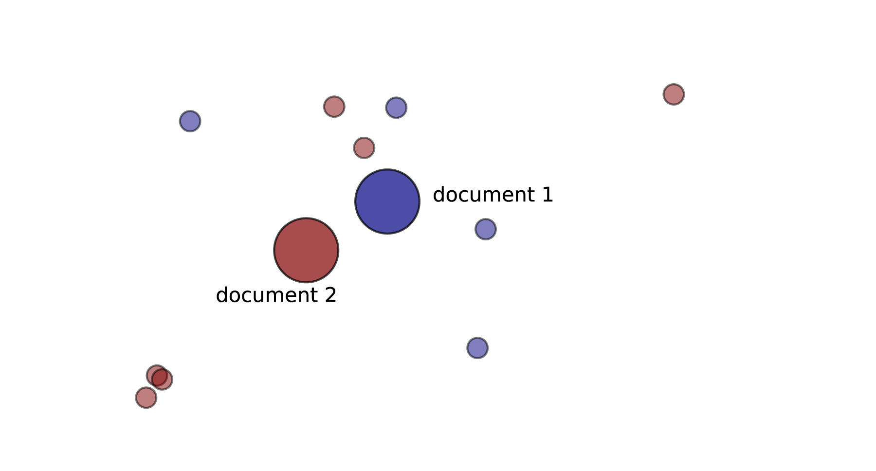
def document_vector(word2vec_model, doc):
    # remove out-of-vocabulary words
    doc = [word for word in doc if word in word2vec_model.vocab]
    return np.mean(word2vec_model[doc], axis=0)
As we cannot compute a mean for a document for which no words is in the word2vec dictionary (the model is not trained on the same corpus, so a word can be missing in the word2vec dictionary), we need to filter our corpus to delete those documents:
def has_vector_representation(word2vec_model, doc):
    """check if at least one word of the document is in the
    word2vec dictionary"""
    return not all(word not in word2vec_model.vocab for word in doc)

corpus, texts, y = filter_docs(corpus, texts, y,
                               lambda doc: has_vector_representation(word2vec_model, doc))

snippets, _, snippets_labels = filter_docs(snippets, None, snippets_labels,
                                                          lambda doc: has_vector_representation(word2vec_model, doc))
We compute a similarity matrix between documents. Each entry of this matrix, sims['ng20']['centroid'][i, j], is the similarity between document i and document j. We are using the cosine similarity between the mean of the word’s vectors of document i and the mean of the word’s vectors of document j.
from sklearn.metrics.pairwise import cosine_similarity

sims['ng20']['centroid'] = cosine_similarity(np.array([document_vector(word2vec_model, doc)
                                                       for doc in corpus]))
Again, a similarity matrix is computed for the web snippets:
sims['snippets']['centroid'] = cosine_similarity(np.array([document_vector(word2vec_model, doc)
                                                           for doc in snippets]))
However, taking the centroid of the words for a document might not capture properly the semantic of the document when some words are far away from each other.
Let’s introduce a more sophisticated method using word embeddings: the Word Mover’s Distance.
Word Mover’s Distance has been introduced in From Word Embeddings To Document Distances, (Kusner et al., ICML 2015).
The following example and illustration (Figure 3) taken from the author Matt Kusner’s website explains the principle. Consider two documents:
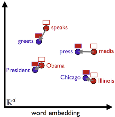
The Word Mover’s Distance is the minimal cumulative distance that the words of the first document need to travel to reach the words of the second document. We take only non-stop words into consideration.
We are using an implementation available as a pull request in gensim. The code is available at https://github.com/olavurmortensen/gensim.
The whole distance matrix can be computed using the following code (warning: this is a very long computation, it took about 26 hours using 6 processors).
from sklearn.metrics.pairwise import pairwise_distances

A = np.array([[i] for i in range(len(snippets))])

def f(x, y):
    return word2vec_model.wmdistance(snippets[int(x)], snippets[int(y)])

X_wmd_distance_snippets = pairwise_distances(A, metric=f, n_jobs=-1)
Now that we have all our models and the distance or similarity matrices (except for the 20 Newsgroups dataset with WMD as it takes too much time), we can evaluate the methods.
First, a local analysis on a single example is done to get a sense of how well the methods work. Then a global analysis is done with a clustering task.
The following code retrieve the top 20 most similar documents for a given query and their similarity score:
def most_similar(i, X_sims, topn=None):
    """return the indices of the topn most similar documents with document i
    given the similarity matrix X_sims"""

    r = np.argsort(X_sims[i])[::-1]
    if r is None:
        return r
    else:
        return r[:topn]

#LSI
print(most_similar(0, sims['ng20']['LSI'], 20))
print(most_similar(0, sims['snippets']['LSI'], 20))

#Centroid
print(most_similar(0, sims['ng20']['centroid'], 20))
print(most_similar(0, sims['snippets']['centroid'], 20))
As we don’t have the similarity matrix for the 20 Newsgroups dataset with the WMD method, we cannot use the same function. We can still compute the distance between all documents and a given query. This method is nevertheless time consuming: it takes about 8 minutes on a laptop (4 cores and 16 GB of RAM) to compute the distances between one document of the 20 Newsgroups dataset and all the others. If we provide a num_best value, an efficient algorithm called « prefetch and prune » is used. It uses a relaxation of the distance computation problem to prune documents that are not in the num_best nearest neighbors, so the computation of the true WMD is not done for these documents. Using this trick, the computation duration is divided by two in this example:
from gensim.similarities import WmdSimilarity

wmd_similarity_top20 = WmdSimilarity(corpus, word2vec_model, num_best=20)
most_similars_wmd_ng20_top20 = wmd_similarity_top20[corpus[0]]
The following code retrieves the top 20 most similar snippets relative to the first one:
wmd_similarity_snippets = WmdSimilarity(snippets, word2vec_model, num_best=20)
most_similars_snippets = wmd_similarity_snippets[snippets[0]]
With this corpus, the WMD is much more usable because the computation time dropped. This is due to the size of the snippets: the best average time complexity of solving the WMD optimization problem scales $O(p^3 \log p)$, where $p$ denotes the number of unique words in the documents.
Here is an illustration of the first three results returned for the snippets. The first line is the query document and the terms in bold are those that are in the query. The index of the snippet is given in brackets. A lemmatization step has been done, and duplicates are removed to make the table readable.
| LSI | Centroid | WMD |
|---|---|---|
| [0] china direcori directori directory- export manufactur product supplier taiwan | [0] china direcori directori directory- export manufactur product supplier taiwan | [0] china direcori directori directory- export manufactur product supplier taiwan |
| [13] directori export manufactur product supplier allproduct buyer com databas global import marketplac volum wholesal | [13] directori export manufactur product supplier allproduct buyer com databas global import marketplac volum wholesal | [13] directori export manufactur product supplier allproduct buyer com databas global import marketplac volum wholesal |
| [973] directori product supplier buyer com commod provid servic sourc trader wand | [15] manufactur product autodesk catalog competit custom design global industri mass mfg outsourc partner partnerproduct reshap servic | [973] directori product supplier buyer com commod provid servic sourc trader wand |
| [2] china manufactur product cost design dfma oversea paper redesign save true truecost | [973] directori product supplier buyer com commod provid servic sourc trader wand | [2] china manufactur product cost design dfma oversea paper redesign save true truecost |
For each corpus, given a single query document (the first of the corpus in this case), we retrieve the top 20 most similar documents with the three methods. A summary of the results is given by the following table:
| Method | Corpus | Query category | Number of documents (out of 20 results) in a different category than the query (categories are given in parentheses) | Comments |
|---|---|---|---|---|
| LSI | ng20 | autos | 2 (forsale and motorcycles) | |
| snippets | business | 7 = 6 (engineering) + 1 (health) | ||
| Centroids method | ng20 | autos | 6 = 2 (politics: guns and mideast) + 4 (motorcycles) | motorcycles is a close category |
| snippets | business | 5 (education-science and engineering) | results are still about manufacturing | |
| WMD | ng20 | autos | 4 (religion, electronics, operating systems, sport) | |
| snippets | business | 6 = 3 (engineering) + 2 (computers) + 1 (health) | results are still about products |
We can see from these results on a single query that LSI seems to be better than the methods using word2vec on the 20 Newsgroups dataset because more retrieved documents belong to the same category as the query. On the snippets dataset, the methods based on word2vec perform well because, even if they don’t always find results from the same category than the query, the results are still related to the query.
In order to confirm (or not) what we have observed in this section, a global evaluation using clustering is performed in the following part.
The clustering task consists in grouping documents into clusters. The documents belonging to the same cluster should be more similar than documents belonging to different clusters. We want the number of clusters to be the same as the number of categories in order to evaluate the results: a cluster should correspond to a category.
As we have the similarity between pairs of documents (except for WMD on the 20 Newsgroups corpus), we are using the spectral clustering algorithm. As we have also the ground truth clusters, we use the Normalized Mutual Information (NMI) criterion to evaluate the quality of this clustering. The spectral clustering algorithm expects as an input a matrix where the values are positives, so we add one to all entries of the similarity matrices (because similarities are by definition lying on the [-1,1] interval).
from sklearn.cluster import SpectralClustering
from sklearn.metrics import normalized_mutual_info_score as nmi

sims['snippets']['WMD'] = -X_wmd_distance_snippets + X_wmd_distance_snippets.max() - 1

for dataset in ['ng20', 'snippets']:
    for method in ['centroid', 'LSI', 'WMD']:
        if not (method == 'WMD' and dataset == 'ng20'):
            if dataset == 'ng20':
                 n_clusters = 20
            else:
                 n_clusters = 8

            sc = SpectralClustering(n_clusters=n_clusters,
                                    affinity='precomputed')

            matrix = sims[dataset][method]
            matrix += 1

            sc.fit(matrix)

            labels = None
            if dataset == 'ng20':
                labels = y
            else:
                labels = snippets_labels

            print("Method: {}\nDataset: {}".format(method, dataset))
            print(nmi(sc.labels_, labels))
            print("-"*10)
The quality of the clustering task for each method is given by the following NMI values:
| LSI | Centroid | WMD | |
|---|---|---|---|
| ng20 | 0.40 | 0.31 | |
| snippets | 0.25 | 0.46 | 0.39 |
LSI is the best method for long texts corresponding to the 20 Newsgroups dataset. This confirms what have been observed on the retrieval task. This is due to the fact that long texts contain more words that co-occur, so a method like LSI have enough information to compute the similarity between documents.
For the Web snippets dataset, WMD and the Centroid method entail both better clustering than LSI. This is due to the lack of co-occurence in small texts. The fact that WMD is worse than the Centroid method for clustering is intriguing. An explanation could be that WMD produce too fine-grained similarity for the clustering task.
Elaborating and computing a similarity measure that captures well the semantic relationships between texts is an important topic given the ubiquity of textual data and the multiple usages it allows: products recommendation, search, sentiment analysis, etc.
In this article, we have seen that using the information given by word2vec in order to compute similarity between textual documents is useful when the documents are small. Taking the centroid of the word vectors for a document is however too limited and performs worse than the commonly used LSI when the documents are large. The sophisticated method WMD is not practical in term of computing time and also, on the corpus we tested, in term of quality.
This leads us to explore other methods in the future: we will try other documents descriptors based on word embeddings in order to handle words corresponding to potentially different topics, and we will try to experiment with words weighting scheme.
